Software Design

Code structure

Castro is built upon the AMReX C++ framework. This provides high-level classes for managing an adaptive mesh refinement simulation, including the core data structures we will deal with. AMReX provides convenient data structures that allow for this workflow—high level objects in C++ that communicate with our computational kernels, with the data regions appearing as multidimensional arrays.

Castro uses a structured-grid approach to hydrodynamics. We work with square/cubic zones that hold state variables (density, momentum, etc.) and compute the fluxes of these quantities through the interfaces of the zones (this is a finite-volume approach). Parallelization is achieved by domain decomposition. We divide our domain into many smaller boxes, and distributed these across processors. When information is needed at the boundaries of the boxes, messages are exchanged and this data is held in a perimeter of ghost cells. AMReX manages this decomposition and communication for us. Additionally, AMReX implements adaptive mesh refinement. In addition to the coarse decomposition of our domain into zones and boxes, we can refine rectangular regions by adding finer-gridded boxes on top of the coarser grid. We call the collection of boxes at the same resolution a level.

Castro uses a hybrid MPI + OpenMP approach to parallelism. MPI is at used to communicate across nodes on a computer and OpenMP is used within a node, to loop over subregions of a box with different threads.

The code structure in the Castro/ directory is:

• Diagnostics/: various analysis routines for specific problems

• Docs/: you’re reading this now!

• Exec/: various problem implementations, sorted by category:

  • gravity_tests/: test problems that primarily exercise the gravity solver

  • hydro_tests/: test problems of the hydrodynamics (with or without reactions)

  • radiation_tests/: test problems that primarily exercise the radiation hydrodynamics solver

  • reacting_tests/: test problems that primarily exercise the reactions (and hydro + reaction coupling)

  • scf_tests/: problem setups that use the self-consistent field initialization

  • science/: problem setups that were used for scientific investigations

  • unit_tests/: test problems that exercise primarily a single module

• external/: if you are using git submodules, the Microphysics and AMReX git submodules will be in this directory.

• paper/: the JOSS paper source

• Source/: source code. In this main directory is all of the code. Sources are organized by topic as:

  • diffusion/ : thermal diffusion code

  • driver/ : the main driver, I/O, runtime parameter support

  • gravity/ : self-gravity code

  • hydro/ : the compressible hydrodynamics code

  • mhd/ : the MHD solver code

  • particles/ : support for particles

  • problems/ : template code for implementing a problem

  • radiation/ : the implicit radiation solve code

  • reactions/ : nuclear reaction code

  • rotation/ : rotating code

  • scf/ : the self-consistent field initialization support

  • sdc/: code specified for the true SDC method

  • sources/ : hydrodynamics source terms support

• Util/: a catch-all for additional things you may need

  • ConvertCheckpoint/: a tool to convert a checkpoint file to a larger domain

  • …

Major data structures

The following data structures are the most commonly encountered when working in the C++ portions of Castro. This are all AMReX data-structures / classes.

Amr

This is the main class that drives the whole simulation. This is the highest level in Castro.

AmrLevel and Castro classes

An AmrLevel is a virtual base class provided by AMReX that stores all the state data on a single level in the AMR hierarchy and understands how to advance that data in time.

The most important data managed by the AmrLevel is an array of StateData, which holds the fluid quantities, etc., in the boxes that together make up the level.

The Castro class is derived from the AmrLevel. It provides the Castro-specific routines to evolve our system of equations. Like the AmrLevel, there is one Castro object for each level in the AMR hierarchry.

A lot of the member data in the Castro class are static member variables—this means that they are shared across all instances of the class. So, in this case, every level will have the same data. This is done, in particular, for the values of the runtime parameters, but also for the Gravity, Diffusion, and Radiation objects. This means that those objects cover all levels and are the same object in each instantiation of the Castro class.

Floating point data

Floating point data in the C++ AMReX framework is declared as Real. This is typedef to either float or double depending on the make variable PRECISION.

Note

single precision support in Castro is not yet complete. In particular, a lot of the supporting microphysics has not been updated.

Box and FArrayBox

A Box is simply a rectangular region in space. It does not hold data. In AMReX, an AMR level has a global index space, with \((0,0,0)\) being the lower left corner of the domain at that level, and \((N_x-1, N_y-1, N_z-1)\) being the upper right corner of the domain (for a domain of \(N_x \times N_y \times N_z\) zones). The location of any Box at a level can be uniquely specified with respect to this global index space by giving the index of its lower-left and upper-right corners. Fig. 1 shows an example of three boxes at the same level of refinement.

AMReX provides other data structures that collect Boxes together, most importantly the BoxArray. We generally do not use these directly, with the exception of the BoxArray grids, which is defined as part of the AmrLevel class that Castro inherits. grids is used when building new MultiFabs to give the layout of the boxes at the current level.

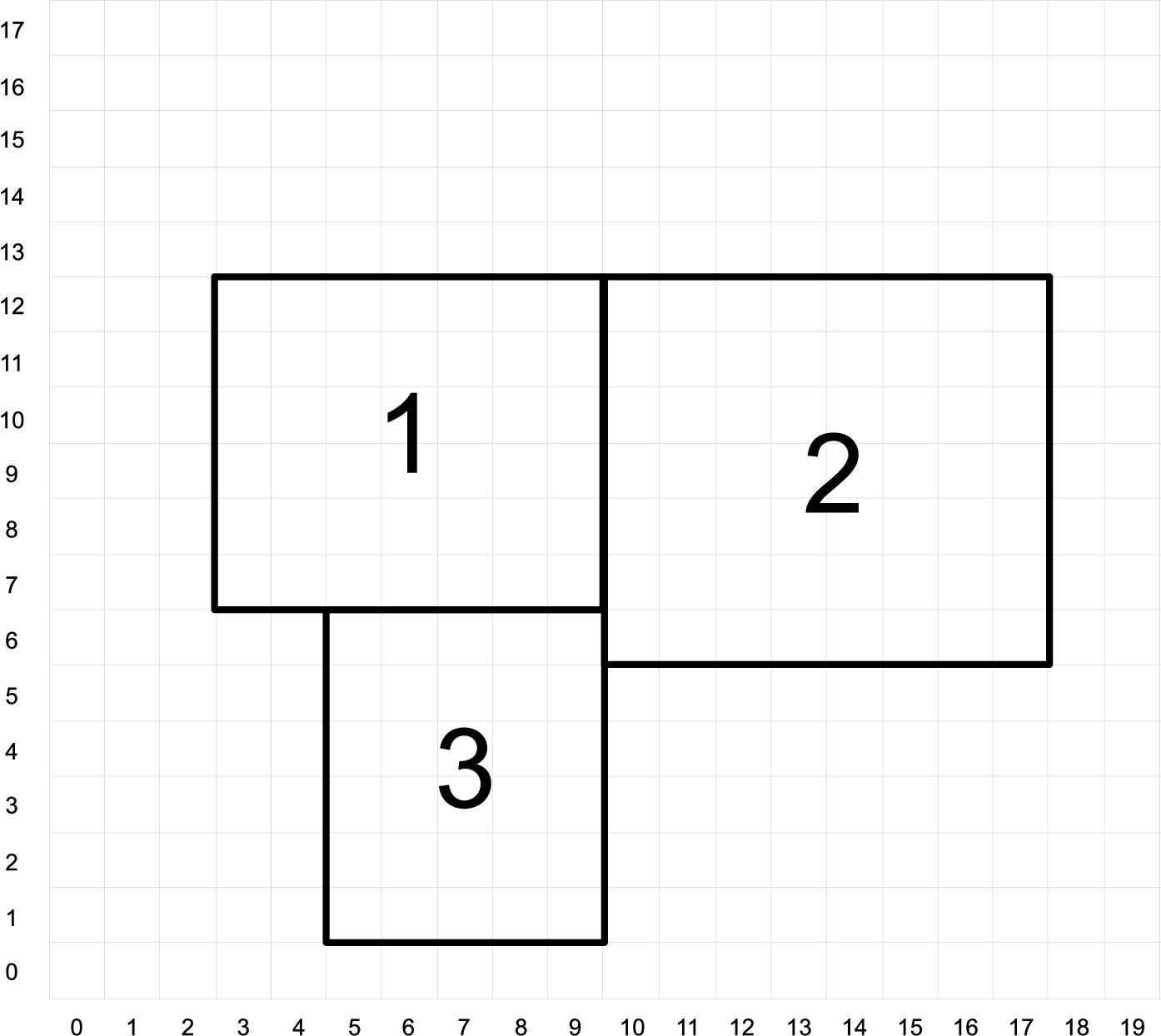
Fig. 1 Three boxes that comprise a single level. At this resolution, the domain is 20 \(\times\) 18 zones. Note that the indexing in AMReX starts with \(0\).

A FArrayBox or FAB, for Fortran array box is a data structure that contains a Box locating it in space, as well as a pointer to a data buffer. The real floating point data are stored as one-dimensional arrays in FArrayBox es. The associated Box can be used to reshape the 1D array into multi-dimensional arrays to be used by Fortran subroutines. The key part of the C++ AMReX data structures is that this data buffer can be cast a a DIM+1 dimensional array that we can easily fill in C++ kernels.

Note

Castro is complied for a specific dimensionality.

MultiFab

At the highest abstraction level, we have the MultiFab (multiple FArrayBoxes). A MultiFab contains an array of Box es, including boxes owned by other processors for the purpose of communication, an array of MPI ranks specifying which MPI processor owns each Box, and an array of pointers to FArrayBoxes owned by this MPI processor.

Note

a MultiFab is a collection of the boxes that together make up a single level of data in the AMR hierarchy.

A MultiFab can have multiple components (like density, temperature, …) as well as a perimeter of ghost cells to exchange data with neighbors or implement boundary conditions (this is all reflected in the underlying FArrayBox).

Parallelization in AMReX is done by distributing the FABs across processors. Each processor knows which FABs are local to it. To loop over all the boxes local to a processor, an MFIter is used (more on this below).

High-level operations exist on MultiFab s to add, subtract, multiply, etc., them together or with scalars, so you don’t need to write out loops over the data directly.

In Castro, MultiFab s are one of the main data structures you will interact with in the C++ portions of the code.

StateData

StateData is a class that essentially holds a pair of MultiFab s: one at the old time and one at the new time. AMReX knows how to interpolate in time between these states to get data at any intermediate point in time. The main data that we care about in Castro (the fluid state, gravitational potential, etc.) will be stored as StateData. Essentially, data is made StateData in Castro if we need it to be stored in checkpoints / plotfiles, and/or we want it to be automatically interpolated when we refine.

An AmrLevel stores an array of StateData (in a C++ array called state). We index this array using integer keys (defined via an enum in Castro.H). The state data is registered with AMReX in Castro_setup.cpp.

Note that each of the different StateData carried in the state array can have different numbers of components, ghost cells, boundary conditions, etc. This is the main reason we separate all this data into separate StateData objects collected together in an indexable array.

The current StateData names Castro carries are:

• State_Type : this is the NUM_STATE hydrodynamics components that make up the conserved hydrodynamics state (usually referred to as \(\Ub\) in these notes. But note that this does not include the radiation energy density.

  We access this data using an AMReX Array4 type which is of the form data(i,j,k,n), where n is the component. The integer keys used to index the components are defined in Source/driver/_variables (e.g., URHO, UMX, UMY, …)

  Note

  regardless of dimensionality, we always carry around all three velocity components. The “out-of-plane” components will simply be advected, but we will allow rotation (in particular, the Coriolis force) to affect them.

  State_Type MultiFab s have no ghost cells.

  Note that the prediction of the hydrodynamic state to the interface will require 4 ghost cells. This accommodated by creating a separate MultiFab, Sborder that lives at the old-time level and has the necessary ghost cells. We will describe this more later.

• Rad_Type : this stores the radiation energy density, commonly denoted \(E_r\) in these notes. It has nGroups components—the number of energy groups used in the multigroup radiation hydrodynamics approximation.

• PhiGrav_Type : this is simply the gravitational potential, usually denoted \(\Phi\) in these notes.

• Gravity_Type : this is the gravitational acceleration. There are always 3 components, regardless of the dimensionality (consistent with our choice of always carrying all 3 velocity components).

• Source_Type : this holds the time-rate of change of the source terms, \(d\Sb/dt\), for each of the NUM_STATE State_Type variables.

  Note

  we do not make use of the old-time quantity here. In fact, we never allocate the FArrayBox s for the old-time in the Source_Type StateData, so there is not wasted memory.

• Reactions_Type : this holds the data for the nuclear reactions. It has NumSpec+2 components: the species creation rates (usually denoted \(\omegadot_k\) in these notes), the specific energy generation rate (\(\dot{e}_\mathrm{nuc}\)), and its density (\(\rho \dot{e}_\mathrm{nuc}\)).

  These are stored as StateData so we have access to the reaction terms outside of advance, both for diagnostics (like flame speed estimation) and for reaction timestep limiting (this in particular needs the data stored in checkpoints for continuity of timestepping upon restart).

• Mag_Type_xthis is defined for MHD and stores the

  face-centered (on x-faces) x-component of the magnetic field.

• Mag_Type_ythis is defined for MHD and stores the

  face-centered (on y-faces) y-component of the magnetic field.

• Mag_Type_zthis is defined for MHD and stores the

  face-centered (on z-faces) z-component of the magnetic field.

• Simplified_SDC_React_Type : this is used with the SDC time-advancement algorithm. This stores the NQSRC terms that describe how the primitive variables change over the timestep due only to reactions. These are used when predicting the interface states of the primitive variables for the hydrodynamics portion of the algorithm.

We access the MultiFab s that carry the data of interest by interacting with the StateData using one of these keys. For instance:

MultiFab& S_new = get_new_data(State_Type);

gets a pointer to the MultiFab containing the hydrodynamics state data at the new time.

MFIter

The process of looping over boxes at a given level of refinement and operating on their data is linked to how Castro achieves thread-level parallelism. The OpenMP approach in Castro has evolved considerably since the original paper was written, with the modern approach, called tiling, gearing up to meet the demands of many-core processors in the next-generation of supercomputers.

Full details of iterating over boxes and calling compute kernels is given in the AMReX documentation here: https://amrex-codes.github.io/amrex/docs_html/Basics.html#mfiter-and-tiling

Practical Details in Working with Tiling

With tiling, the OpenMP is now all at the loop over boxes and not in the computational kernels themselves.

It is the responsibility of the coder to make sure that the routines within a tiled region are safe to use with OpenMP. In particular, note that:

• tile boxes are non-overlapping

• the union of tile boxes completely cover the valid region of the fab

• Consider working with a node-centered MultiFab, ugdnv, and a cell-centered MultiFab s:

  • with mfi(s), the tiles are based on the cell-centered index space. If you have an \(8\times 8\) box, then and 4 tiles, then your tiling boxes will range from \(0\rightarrow 3\), \(4\rightarrow 7\).

  • with mfi(ugdnv), the tiles are based on nodal indices, so your tiling boxes will range from \(0\rightarrow 3\), \(4\rightarrow 8\).

• When updating routines to work with tiling, we need to understand the distinction between the index-space of the entire box (which corresponds to the memory layout) and the index-space of the tile.

Boundaries: FillPatch and FillPatchIterator

AMReX calls the act of filling ghost cells a fillpatch operation. Boundaries between grids are of two types. The first we call “fine-fine”, which is two grids at the same level. The second type is “coarse-fine”, which needs interpolation from the coarse grid to fill the fine grid ghost cells. Both of these are part of the fillpatch operation. Fine-fine fills are just a straight copy from “valid regions” to ghost cells. Coarse-fine fills are enabled because the StateData is not just arrays, they’re “State Data”, which means that the data knows how to interpolate itself (in an anthropomorphical sense). The type of interpolation to use is defined in Castro_setup.cpp—search for cell_cons_interp, for example—that’s “cell conservative interpolation”, i.e., the data is cell-based (as opposed to node-based or edge-based) and the interpolation is such that the average of the fine values created is equal to the coarse value from which they came. (This wouldn’t be the case with straight linear interpolation, for example.)

Additionally, since StateData has an old and new timelevel, the fill patch operation can interpolate to an intermediate time.

Examples

To illustrate the various ways we fill ghost cells and use the data, let’s consider the following scenarios:

• You have state data that was defined with no ghost cells. You want to create a new MultiFab containing a copy of that data with NGROW ghost cells.

  This is the case with Sborder —the MultiFab of the hydrodynamic state that we use to kick-off the hydrodynamics advance.

  Sborder is declared in Castro.H simply as:

  Multifab Sborder;
  

  It is then allocated in Castro::initialize_do_advance()

  Sborder.define(grids, NUM_STATE, NUM_GROW, Fab_allocate);
  const Real prev_time = state[State_Type].prevTime();
  expand_state(Sborder, prev_time, NUM_GROW);
  

  Note in the call to .define(), we tell AMReX to already allocate the data regions for the FArrayBox s that are part of Sborder.

  The actually filling of the ghost cells is done by Castro::expand_state():

  AmrLevel::FillPatch(*this, Sborder, NUM_GROW,
                      prev_time, State_Type, 0, NUM_STATE);
  

  Here, we are filling the ng ghost cells of MultiFab Sborder at time prev_time. We are using the StateData that is part of the current Castro object that we are part of. Note: FillPatch takes an object reference as its first argument, which is the object that contains the relevant StateData —that is what the this pointer indicates. Finally, we are copying the State_Type data components 0 to NUM_STATE [1].

  The result of this operation is that Sborder will now have NUM_GROW ghost cells consistent with the State_Type data at the old time-level.

• You have state data that was defined with NGROW ghost cells. You want to ensure that the ghost cells are filled (including any physical boundaries) with valid data.

  This is very similar to the procedure shown above. The main difference is that for the MultiFab that will be the target of the ghost cell filling, we pass in a reference to the StateData itself.

  The main thing you need to be careful of here, is that you need to ensure that the the time you are at is consistent with the StateData ’s time. Here’s an example from the radiation portion of the code MGFLDRadSolver.cpp:

  Real time = castro->get_state_data(Rad_Type).curTime();
  MultiFab& S_new = castro->get_new_data(State_Type);
  
  AmrLevel::FillPatch(*castro, S_new, ngrow, time, State_Type,
                      0, S_new.nComp(), 0);
  

  In this example, S_new is a pointer to the new-time-level State_Type MultiFab. So this operation will use the State_Type data to fill its own ghost cells. we fill the ngrow ghost cells of the new-time-level State_Type data, for all the components.

  Note that in this example, because the StateData lives in the castro object and we are working from the Radiation object, we need to make reference to the current castro object pointer. If this were all done within the castro object, then the pointer will simply be this, as we saw above.

• You have a MultiFab with some derived quantity. You want to fill its ghost cells.

  MultiFabs have a FillBoundary() method that will fill all the ghost cells between boxes at the same level. It will not fill ghost cells at coarse-fine boundaries or at physical boundaries.

• You want to loop over the FABs in state data, filling ghost cells along the way

  This is the job of the FillPatchIterator—this iterator is used to loop over the grids and fill ghostcells. A key thing to keep in mind about the FillPatchIterator is that you operate on a copy of the data—the data is disconnected from the original source. If you want to update the data in the source, you need to explicitly copy it back. Also note: FillPatchIterator takes a MultiFab, but this is not filled—this is only used to get the grid layout. Finally, the way the FillPatchIterator is implemented is that all the communication is done first, and then the iterating over boxes commences.

  For example, the loop that calls CA_UMDRV (all the hydrodynamics integration stuff) starts with:

  for (FillPatchIterator fpi(*this, S_new, NUM_GROW,
                             time, State_Type, strtComp, NUM_STATE);
        fpi.isValid(); ++fpi)
  {
    FArrayBox &state = fpi();
    Box bx(fpi.validbox());
  
    // work on the state FAB.  The interior (valid) cells will
    // live between bx.loVect() and bx.hiVect()
  }
  

  Here the FillPatchIterator is the thing that distributes the grids over processors and makes parallel “just work”. This fills the single patch fpi , which has NUM_GROW ghost cells, with data of type State_Type at time time, starting with component strtComp and including a total of NUM_STATE components.

In general, one should never assume that ghostcells are valid, and instead do a fill patch operation when in doubt. Sometimes we will use a FillPatchIterator to fill the ghost cells into a MultiFab without an explicit look. This is done as:

FillPatchIterator fpi(*this,S_old,1,time,State_Type,0,NUM_STATE);
MultiFab& state_old = fpi.get_mf();

In this operation, state_old points to the internal MultiFab in the FillPatchIterator, by getting a reference to it as fpi.get_mf(). This avoids a local copy.

Note that in the examples above, we see that only StateData can fill physical boundaries (because these register how to fill the boundaries when they are defined). There are some advanced operations in AMReX that can get around this, but we do not use them in Castro.

Physical Boundaries

Physical boundary conditions are specified by an integer index [2] in the inputs file, using the castro.lo_bc and castro.hi_bc runtime parameters. Table Table 5 shows the correspondence between the integer key and the physical assumption, as well as the action each takes for the normal velocity, transverse velocity, and generic scalar.

Table 5 Physical boundary conditions supported in Castro.

name	integer	normal velocity	transverse velocity	scalars
interior	0	BCType::int_dir	BCType::int_dir	BCType::int_dir
inflow	1	BCType::ext_dir	BCType::ext_dir	BCType::ext_dir
outflow	2	BCType::foextrap	BCType::foextrap	BCType::foextrap
symmetry	3	BCType::reflect_odd	BCType::reflect_even	BCType::reflect_even
slipwall	4	BCType::reflect_odd	BCType::reflect_even	BCType::reflect_even
noslipwall	5	BCType::reflect_odd	BCType::reflect_even	BCType::reflect_even

The definition of the specific actions are:

• BCType::int_dir: data taken from other grids or interpolated

• BCType::ext_dir: data specified on EDGE (FACE) of boundary

• BCType::hoextrap: higher order extrapolation to EDGE of boundary

• BCType::foextrap: first order extrapolation from last cell in interior

• BCType::reflect_even: \(F(-n) = F(n)\) true reflection from interior cells

• BCType::reflect_odd: \(F(-n) = -F(n)\) true reflection from interior cells

The actual registration of a boundary condition action to a particular variable is done in Castro_setup.cpp. At the top we define arrays such as scalar_bc, norm_vel_bc, etc, which say which kind of bc to use on which kind of physical boundary. Boundary conditions are set in functions like set_scalar_bc, which uses the scalar_bc pre-defined arrays. We also specify the name of the routine that is responsible for filling the data there (e.g., hypfill). These routines are discussed more below.

If you want to specify a value at a function (like at an inflow boundary), then you choose an inflow boundary at that face of the domain. You then need to write the implementation code for this. There is a centralized hydrostatic boundary condition that is implemented this way—see Boundary Conditions.

FluxRegister

A FluxRegister holds face-centered data at the boundaries of a box. It is composed of a set of MultiFab s (one for each face, so 6 for 3D). A FluxRegister stores fluxes at coarse-fine interfaces, and isused for the flux-correction step.

Other AMReX Concepts

There are a large number of classes that help define the structure of the grids, metadata associate with the variables, etc. A good way to get a sense of these is to look at the .H files in the amrex/Src/ directory.

Geometry class

There is a Geometry object, geom for each level as part of the Castro object (this is inherited through AmrLevel).

ParmParse class

Error Estimators

Gravity class

There is a single Gravity object, gravity, that is a static class member of the Castro object. This means that all levels refer to the same Gravity object.

Within the Gravity object, there are pointers to the Amr object (as parent), and all of the AmrLevels (as a PArray, LevelData). The gravity object gets the geometry information at each level through the parent Amr class.

The main job of the gravity object is to provide the potential and gravitation acceleration for use in the hydrodynamic sources. Depending on the approximation used for gravity, this could mean calling the AMReX multigrid solvers to solve the Poisson equation.

[1]

for clarity and continuity in this documentation, some of the variable names have been changed compared to the actual code

[2]

the integer values are defined in BC_TYPES.H