Integrating a Network
Reaction ODE System
Note
This describes the integration done when doing Strang operator-splitting, which is the default mode of coupling burning to application codes.
The equations we integrate to do a nuclear burn are:
Here, \(X_k\) is the mass fraction of species \(k\), \(e\) is the specific nuclear energy created through reactions. Also needed are density \(\rho\), temperature \(T\), and the specific heat. The function \(f\) provides the energy release from reactions and can often be expressed in terms of the instantaneous reaction terms, \(\dot{X}_k\). As noted in the previous section, this is implemented in a network-specific manner.
In this system, \(e\) is equal to the total specific internal energy. This allows us to easily call the EOS during the burn to obtain the temperature.
Note
The energy generation rate includes a term for neutrino losses in addition to the energy release from the changing binding energy of the fusion products.
While this is the most common way to construct the set of burn equations, and is used in most of our production networks, all of them are ultimately implemented by the network itself, which can choose to disable the evolution of any of these equations by setting the RHS to zero. The integration software provides some helper routines that construct common RHS evaluations, like the routine that converts a temperature update to \(\dot{e}\), but these calls are always explicitly done by the individual networks rather than being handled by the integration backend. This allows you to write a new network that defines the RHS in whatever way you like.
The standard reaction rates can all be boosted by a constant factor by
setting the react_boost runtime parameter. This will simply
multiply the righthand sides of each species evolution equation (and
appropriate Jacobian terms) by the specified constant amount.
Interfaces
The interfaces to all of the networks and integrators are written in C++.
burner
The main entry point for C++ is burner() in
interfaces/burner.H. This simply calls the integrator()
routine (at the moment this can be VODE, BackwardEuler, ForwardEuler, QSS, or RKC).
AMREX_GPU_HOST_DEVICE AMREX_FORCE_INLINE
void burner (burn_t& state, Real dt)
The input is a burn_t.
Note
For the thermodynamic state, only the density, temperature, and mass fractions are used directly–we compute the internal energy corresponding to this input state through the equation of state before integrating.
When integrating the system, we often need auxiliary information to
close the system. This is kept in the original burn_t that was
passed into the integration routines. For this reason, we often need
to pass both the specific integrator’s type (e.g. dvode_t) and
burn_t objects into the lower-level network routines.
The overall flow of the integrator is (using VODE as the example):
Call the EOS directly on the input
burn_tstate using \(\rho\) and \(T\) as inputs.Fill the integrator type by calling
burn_to_integrator()to create advode_t.call the ODE integrator,
dvode(), passing in thedvode_t_and_ theburn_t— as noted above, the auxiliary information that is not part of the integration state will be obtained from theburn_t.subtract off the energy offset—we now store just the energy released in the
dvode_tintegration state.convert back to a
burn_tby callingintegrator_to_burnnormalize the abundances so they sum to 1.
Note
Upon exit, burn_t burn_state.e is the energy released during
the burn, and not the actual internal energy of the state.
Optionally, by setting integrator.subtract_internal_energy=0
the output will be the total internal energy, including that released
burning the burn.
Network Routines
Note
Microphysics integrates the reaction system in terms of mass fractions, \(X_k\), but most astrophysical networks use molar fractions, \(Y_k\). As a result, we expect the networks to return the righthand side and Jacobians in terms of molar fractions. The integration wrappers will internally convert to mass fractions as needed for the integrators.
Righthand size implementation
The righthand side of the network is implemented by
actual_rhs() in actual_rhs.H, and appears as
void actual_rhs(burn_t& state, Array1D<Real, 1, neqs>& ydot)
All of the necessary integration data comes in through state, as:
state.xn[NumSpec]: the mass fractions.state.aux[NumAux]: the auxiliary data (only available ifNAUX_NET> 0)state.e: the current internal energy. It is very rare (never?) that a RHS implementation would need to use this variable directly – even though this is the main thermodynamic integration variable, we obtain the temperature from the energy through an EOS evaluation.state.T: the current temperaturestate.rho: the current density
Note that we come in with the mass fractions, but the molar fractions can be computed as:
Array1D<Real, 1, NumSpec> y;
...
for (int i = 1; i <= NumSpec; ++i) {
    y(i) = state.xn[i-1] * aion_inv[i-1];
}
Note
We use 1-based indexing for ydot for legacy reasons, so watch out when filling in
this array based on 0-indexed C arrays.
The actual_rhs() routine’s job is to fill the righthand side vector
for the ODE system, ydot(neqs). Here, the important
fields to fill are:
state.ydot(1:NumSpec): the change in molar fractions for theNumSpecspecies that we are evolving, \(d({Y}_k)/dt\)state.ydot(net_ienuc): the change in the internal energy from the net, \(de/dt\)
The righthand side routine is assumed to return the change in molar fractions, \(dY_k/dt\). These will be converted to the change in mass fractions, \(dX_k/dt\) by the wrappers that call the righthand side routine for the integrator. If the network builds the RHS in terms of mass fractions directly, \(dX_k/dt\), then these will need to be converted to molar fraction rates for storage, e.g., \(dY_k/dt = A_k^{-1} dX_k/dt\).
Righthand side wrapper
The integrator provides a wrapper that sits between the integration routines and the network’s implementation of the righthand side. Its flow is (for VODE):
call
clean_stateon thedvode_tupdate the thermodynamics by calling
update_thermodynamics. This takes both thedvode_tand theburn_tand computes the temperature that matches the current state.call
actual_rhsconvert the derivatives to mass-fraction-based (since we integrate \(X\)) and zero out the temperature and energy derivatives if we are not integrating those quantities.
apply any boosting if
react_boost> 0
Jacobian implementation
The Jacobian is provided by actual_jac(state, jac), and takes the
form:
void actual_jac(burn_t& state, MathArray2D<1, neqs, 1, neqs>& jac)
The Jacobian matrix elements are stored in jac as:
jac(m, n)for \(\mathrm{m}, \mathrm{n} \in [1, \mathrm{NumSpec}]\) : \(d(\dot{Y}_m)/dY_n\)jac(net_ienuc, n)for \(\mathrm{n} \in [1, \mathrm{NumSpec}]\) : \(d(\dot{e})/dY_n\)jac(m, net_ienuc)for \(\mathrm{m} \in [1, \mathrm{NumSpec}]\) : \(d(\dot{Y}_m)/de\)jac(net_ienuc, net_ienuc): \(d(\dot{e})/de\)
The form looks like:
Note: a network is not required to compute a Jacobian if a numerical
Jacobian is used. This is set with the runtime parameter
jacobian = 2, and implemented directly in VODE or via
integration/utils/numerical_jacobian.H for other integrators.
Jacobian wrapper
The integrator provides a wrapper that sits between the integration routines and the network’s implementation of the Jacobian. Its flow is (for VODE):
Note
It is assumed that the thermodynamics are already correct when
calling the Jacobian wrapper, likely because we just called the RHS
wrapper above which did the clean_state and
update_thermodynamics calls.
call
integrator_to_burnto update theburn_tcall
actual_jac()to have the network fill the Jacobian arrayconvert the derivative to be mass-fraction-based
apply any boosting to the rates if
react_boost> 0
Thermodynamics and \(e\) Evolution
The thermodynamic equation in our system is the evolution of the internal energy, \(e\). (Note: when the system is integrated in an operator-split approach, this responds only to the nuclear energy release and not pdV work.)
At initialization, \(e\) is set to the value from the EOS consistent with the initial temperature, density, and composition:
In the integration routines, this is termed the “energy offset”.
As the system is integrated, \(e\) is updated to account for the nuclear energy release,
Upon exit, we subtract off this initial offset, so state.e in
the returned burn_t type from the actual_integrator
call represents the energy release during the burn.
Integration of Equation (2) requires an evaluation of the temperature at each integration step (since the RHS for the species is given in terms of \(T\), not \(e\)). This involves an EOS call and is the default behavior of the integration.
If desired, the EOS call can be skipped and the temperature kept
frozen over the entire time interval of the integration. This is done
by setting integrator.call_eos_in_rhs = 0.
Note also that for the Jacobian, we need the specific heat, \(c_v\), since we
usually calculate derivatives with respect to temperature (as this is the form
the rates are commonly provided in). We use the specific heat at constant volume
because it is most consistent with the operator split methodology we use (density
is held constant during the burn when doing Strang splitting).
Similar to temperature, this will automatically be updated at each integration
step (unless you set integrator.call_eos_in_rhs = 0).
Renormalization
The renormalize_abundances parameter controls whether we
renormalize the abundances so that the mass fractions sum to one
during a burn. This has the positive benefit that in some cases it can
prevent the integrator from going off to infinity or otherwise go
crazy; a possible negative benefit is that it may slow down
convergence because it interferes with the integration
scheme. Regardless of whether you enable this, we will always ensure
that the mass fractions stay positive and larger than some floor
small_x.
Stiff ODE Solvers
We use a high-order implicit ODE solver for integrating the reaction
system. A few alternatives, including first order implicit and explicit integrators are also
provided. Internally, the integrators use different data structures
to store the integration progress, and each integrator needs to
provide a routine to convert from the integrator’s internal
representation to the burn_t type required by the actual_rhs
and actual_jac routine.
The name of the integrator can be selected at compile time using
the INTEGRATOR_DIR variable in the makefile. Presently,
the allowed options are:
BackwardEuler: an implicit first-order accurate backward-Euler method. An error estimate is done by taking 2 half steps and comparing to a single full step. This error is then used to control the timestep by using the local truncation error scaling.ForwardEuler: an explicit first-order forward-Euler method. This is meant for testing purposes only. No Jacobian is needed.QSS: the quasi-steady-state method of [MOvanLeer00] (see also [GH13]). This uses a second-order predictor-corrector method, and is designed specifically for handling coupled ODE systems for chemical and nuclear reactions. However, this integrator has difficulty near NSE, so we don’t recommend its use in production for nuclear astrophysics.
RKC: a stabilized explicit Runge-Kutta-Chebyshev integrator based on [SSV98]. This does not require a Jacobian, but does need to estimate the spectral radius of the system, which is done internally. This works for moderately stiff problems.The spectral radius is estimated by default using the power method, built into RKC. Alternately, by setting
integrator.use_circle_theorem=1, the Gershgorin circle theorem is used instead.VODE: the VODE [BBH89] integration package. We ported this integrator to C++ and removed the non-stiff integration code paths.
We recommend that you use the VODE solver, as it is the most robust.
Important
The integrator will not abort if it encounters trouble. Instead it will
set burn_t burn_state.success = false on exit. It is up to the
application code to handle the failure.
Note
The runtime parameter integrator.scale_system
will scale the internal energy that the integrator sees by the initial
value of \(e\) to make the system \(\mathcal{O}(1)\). The value
of atol_enuc will likewise be scaled. This works for both Strang
and simplified-SDC. For the RKC integrator, this is enabled by
default.
For most integrators this algebraic change should not affect the output to more than roundoff, but the option is included to allow for some different integration approaches in the future.
This option currently does not work with the ForwardEuler or QSS integrators.
Tolerances
Tolerances dictate how accurate the ODE solver must be while solving
equations during a simulation. Typically, the smaller the tolerance
is, the more accurate the results will be. However, if the tolerance
is too small, the code may run for too long or the ODE solver will
never converge. In these simulations, rtol values will set the
relative tolerances and atol values will set the absolute tolerances
for the ODE solver. Often, one can find and set these values in an
input file for a simulation.
Fig. 1 shows the results of a simple simulation using the burn_cell unit test to determine what tolerances are ideal for simulations. For this investigation, it was assumed that a run with a tolerance of \(10^{-12}\) corresponded to an exact result, so it is used as the basis for the rest of the tests. From the figure, one can infer that the \(10^{-3}\) and \(10^{-6}\) tolerances do not yield the most accurate results because their relative error values are fairly large. However, the test with a tolerance of \(10^{-9}\) is accurate and not so low that it takes incredible amounts of computer time, so \(10^{-9}\) should be used as the default tolerance in future simulations.
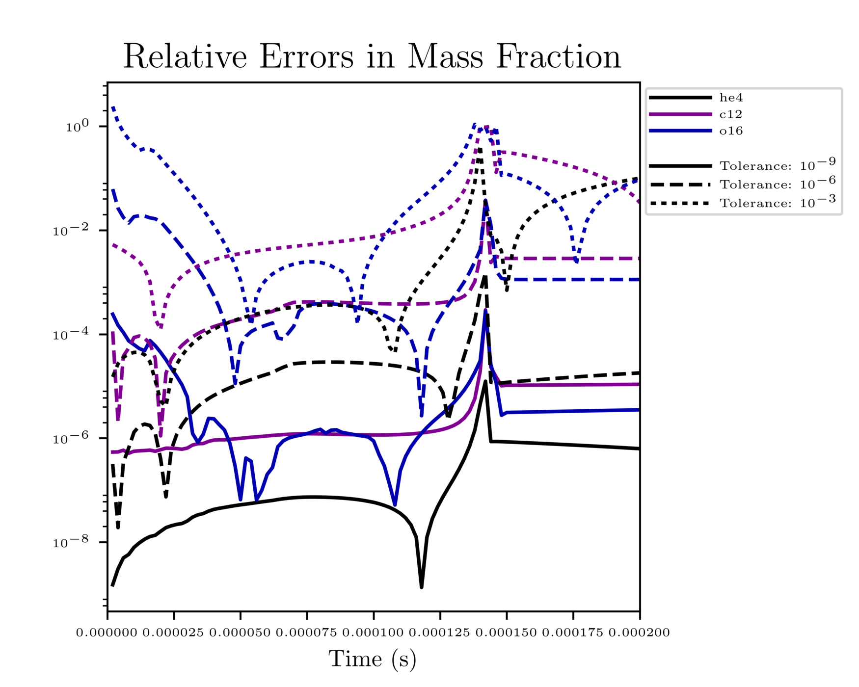
Fig. 1 Relative error of runs with varying tolerances as compared to a run with an ODE tolerance of \(10^{-12}\).
The integration tolerances for the burn are controlled by
rtol_spec and rtol_enuc,
which are the relative error tolerances for
(1) and (2),
respectively. There are corresponding
atol parameters for the absolute error tolerances. Note that
not all integrators handle error tolerances the same way—see the
sections below for integrator-specific information.
The absolute error tolerances are set by default to \(10^{-12}\) for the species, and a relative tolerance of \(10^{-6}\) is used for the temperature and energy.
Overriding Parameter Defaults on a Network-by-Network Basis
Any network can override or add to any of the existing runtime
parameters by creating a _parameters file in the network directory
(e.g., networks/triple_alpha_plus_cago/_parameters). As noted in
Chapter [chapter:parameters], the fourth column in the _parameter
file definition is the priority. When a duplicate parameter is
encountered by the scripts writing the runtime parameter header files, the value
of the parameter with the highest priority is used. So picking a large
integer value for the priority in a network’s _parameter file will
ensure that it takes precedence.