Introduction
A large number of interesting astrophysical phenomena
occur at low Mach numbers. Evolving these flows with a
fully compressible simulation code is inefficient,
because of the need to follow the sound waves. For an
explicit time-discretization (i.e., the new state is
expressed solely in terms of the present state), a
fundamental limitation exists on the size of the
allowable timesteps -- the CFL condition. A timestep is
restricted such that information may only propagate
across one zone in the computational grid per timestep.
In compressible flow, information propagates at the
speeds: u,
MAESTROeX solves a reformulation of the equations of hydrodynamics that filters out sound waves, while retaining the compressibility effects important to the problem at hand. This results in a timestep constraint of the form Δ t < min{ Δ x / |u| } Therefore, MAESTROeX requires far fewer timesteps (~1/M fewer) to simulate low Mach number flows.
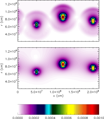
Figure 1: Mach number for 3 burning rising bubbles from a compressible code (top) and a low Mach number hydrodynamics method (bottom).
Mathematically, we can think of low Mach number flows
as exhibiting instantaneous acoustic equilibriation.
Figure 1 shows this graphically. Three temperature
perturbations were placed in a stratified atmosphere,
seeding nuclear reactions. The heat release makes the
bubbles buoyant. The top panel shows the Mach number
for the compressible solution—a clear signal
resulting from the finite propagation speed of the
soundwaves is seen surrounding each bubble. In the low
panel, a low Mach number method was used. Owing to the
instantaneous acoustic equilibriation, the velocity
field is realized throughout the whole domain—even
far from the bubbles. However, the flow at the bubbles
is identical between the two codes, showing that in this
case, the soundwaves are not imporatant to the dynamics.
Low Mach number variations
There are several popular methods for filtering soundwaves, which we summarize below.
Incompressible hydrodynamics
The simplest low Mach number approximation is incompressible hydrodynamics. This approximation is formally the M → 0 limit of the Navier-Stokes equations. In incompressible hydrodynamics, the velocity satisfies a constraint equation ∇ ⋅ U = 0 which acts to instantaneously equilibrate the flow, thereby filtering out soundwaves.
The constraint equation implies that Dρ/Dt = 0 which says that the density is constant along particle paths. This means that there are no compressibility effects modeled in this approximation.
Anelastic hydrodynamics
In the anelastic approximation small amplitude thermodynamic perturbations are carried with respect to a hydrostatic background. The density perturbation is ignored in the continuity equation, resulting in a constraint equation ∇ ⋅ (ρ0U) = 0 This properly captures the compressibility effects due to the stratification of the background. Because there is no evolution equation for the perturbational density, approximations are made to the buoyancy term in the momentum equation.
The low Mach number combustion model
In the low Mach number combustion model, the pressure is decomposed into a dynamic, π, and thermodynamic component, p0, the ratio of which is O(M2). The total pressure is replaced everywhere by the thermodynamic pressure, except in the momentum equation. This decouples the pressure and density and filters out the sound waves. Large amplitude density and temperature fluctuations are allowed. The only requirement is that the total pressure stay close to the background pressure, which is assumed constant. This requirement can be expressed as p = p0, and differentiating this along particle paths leads to a constraint on the velocity field: ∇ ⋅ U = S This looks like the constraint for incompressible hydrodynamics, but now we have a source term, S, representing the compressibility effects due to the energy generation and thermal diffusion.
Since the background pressure is taken to be constant, we cannot model flows that cover a large fraction of a pressure scale height. However, this method is ideal for exploring the physics of flames. We formulated this algorithm for astrophysical flows and used it to explore the dynamics of Rayleigh-Taylor unstable flame fronts in Type Ia supernovae in two- and three-dimensions. This was the predecessor to Maestro.
Low Mach number stellar flows
To model the full star, we begin with the low Mach
number combustion model described above, but no longer
assume that the background pressure is constant, but
instead, is hydrostatically stratified. This results in
a constraint on the velocity field of:
∇ ⋅ ( β0U) = β0[
S - 1/(Γ1p0)
∂p0/∂t]
Here, β0 is a density-like variable.
Again, large amplitude density and temperature
variations are allowed. The only restriction is that
the pressure remain close to the background pressure.
In the presence of heating, the star will expand, and
therefore we need to evolve the background state in
response to the local heating. This is an
extension of the pseudo-incompressible method introduced
in the atmospheric science community. As with anelastic
hydrodynamics, this constraint incorporates the effects
of the background stratification. However, in contrast
to anelastic, the right-hand side is non-zero, and
represents the compressibility effects due to heating
and the change in the background state.
microphysics
A default γ-law equation of state and
general-composition non-reacting network as distributed
in the main MAESTROeX git repo. Additional equations of
state (including a general stellar EOS) and many nuclear
reaction networks are distributed in
the Microphysics
git repo. Maintaining them in a separate repo allows all of the
AMReX astrophysics codes share the same microphysics.
reproducibility
All MAESTROeX plotfiles store information about the build environment (build machine, build date, compiler version and flags), run environment (output date, output dir, number of processors, wall clock time), and code versions used (git hashes for the main MAESTROeX source and AMReX source, and support repos, if available). This allows for a recovery of the code base used for previous results.
MAESTROeX is run through a nightly regression test suite that checks the output, bit-for-bit, against stored benchmarks for many of the problem setups (including real science runs).
parallel performance
coming soon...