Available Reaction Networks
A network defines the composition, which is needed by the equation of state and transport coefficient routines. Even if there are no reactions taking place, a network still needs to be defined, so Microphysics knows the properties of the fluid.
Note
The network is set at compile-time via the NETWORK_DIR
make variable.
Tip
If reactions can be ignored, then the general_null network can
be used — this simply defines a composition with no reactions.
Tip
Many of the networks here are generated using pynucastro [19, 20] using the AmrexAstroCxxNetwork
class.
Each of these networks has a python script that generates the
network (through a function called create_network(). The script
is named after the network. This allows us to recreate the
network in a python environment easily to explore the network flow
from a simulation. For example, to load the CNO_extras network,
we can do:
import os
from pathlib import Path
import sys

mp = os.getenv("MICROPHYSICS_HOME")
moddir = Path(mp) / "networks" / "CNO_extras"
sys.path.insert(0, str(moddir))

import CNO_extras as pynet
net = pynet.create_network()
You can then work with the network through the net object, for instance
using net.plot() to plot the rate strengths at a particular set of
thermodynamic conditions.
general_null
general_null is a bare interface for a nuclear reaction network —
no reactions are enabled. The
data in the network is defined at compile type by specifying an
inputs file. For example,
networks/general_null/triple_alpha_plus_o.net would describe the
triple-\(\alpha\) reaction converting helium into carbon, as
well as oxygen and iron. This has the form:
# name       short name    aion     zion
helium-4       He4          4.0      2.0
carbon-12      C12         12.0      6.0
oxygen-16      O16         16.0      8.0
iron-56        Fe56        56.0     26.0
The four columns give the long name of the species, the short form that will be used for plotfile variables, and the mass number, \(A\), and proton number, \(Z\).
The name of the inputs file by one of two make variables:
NETWORK_INPUTS: this is simply the name of the “.net” file, without any path. The build system will look for it in the current directory and then in$(MICROPHYSICS_HOME)/networks/general_null/.For the example above, we would set:
NETWORK_INPUTS := triple_alpha_plus_o.net
GENERAL_NET_INPUTS: this is the full path to the file. For example we could set:GENERAL_NET_INPUTS := /path/to/file/triple_alpha_plus_o.net
At compile time, the “.net” file is parsed and a network header
network_properties.H is written using the python script
write_network.py. The make rule for this is contained in
Microphysics/networks/Make.package.
iso7, aprox13, aprox19, and aprox21
These are alpha-chains (with some other nuclei) based on the original
Fortran networks from Frank Timmes. These
networks share common rates from Microphysics/rates and are
implemented using the templated C++ network infrastructure.
These networks approximate a lot of the links, in particular, combining \((\alpha, p)(p, \gamma)\) and \((\alpha, \gamma)\) into a single effective rate.
The available networks are:
iso7: contains \(\isotm{He}{4}\), \(\isotm{C}{12}\), \(\isotm{O}{16}\), \(\isotm{Ne}{20}\), \(\isotm{Mg}{24}\), \(\isotm{Si}{28}\), \(\isotm{Ni}{56}\) and is based on [21].aprox13: adds \(\isotm{S}{32}\), \(\isotm{Ar}{36}\), \(\isotm{Ca}{40}\), \(\isotm{Ti}{44}\), \(\isotm{Cr}{48}\), \(\isotm{Fe}{52}\)aprox19: adds \(\isotm{H}{1}\), \(\isotm{He}{3}\), \(\isotm{N}{14}\), \(\isotm{Fe}{54}\), \(\mathrm{p}\), \(\mathrm{n}\). Here, \(\mathrm{p}\) participates only in the photodisintegration rates at high mass number, and is distinct from \(\isotm{H}{1}\).aprox21: adds \(\isotm{Cr}{56}\), \(\isotm{Fe}{56}\). This is designed to reach a lower \(Y_e\) than the other networks, for use in massive star simulations. Note that the link to \(\isotm{Cr}{56}\) is greatly approximated.
These networks store the total binding energy of the nucleus in MeV as
bion(:). They then compute the mass of each nucleus in grams as:
where \(m_n\), \(m_p\), and \(m_e\) are the neutron, proton, and electron
masses, \(A_k\) and \(Z_k\) are the atomic weight and number, and \(B_k\)
is the binding energy of the nucleus (converted to grams). \(M_k\)
is stored as mion(:) in the network.
The energy release per gram is converted from the rates as:
where \(N_A\) is Avogadro’s number (to convert this to “per gram”) and \(\epsilon_\nu\) is the neutrino loss term (see Neutrino Losses).
CNO_extras
This network replicates the popular MESA “cno_extras” network which is meant to study hot-CNO burning and the start of the breakout from CNO burning. This network is managed by pynucastro.
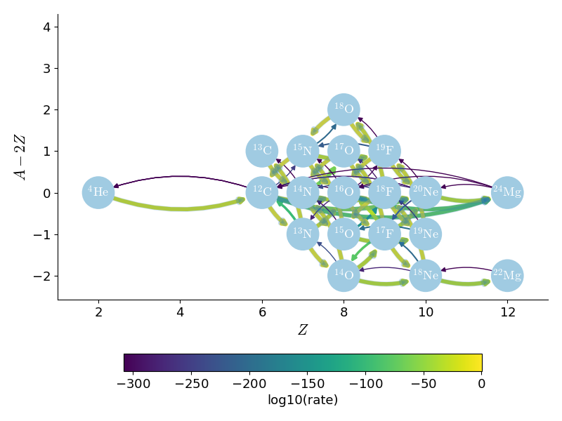
Note
We add \({}^{56}\mathrm{Fe}\) as an inert nucleus to allow this to be used for X-ray burst simulations (not shown in the network diagram above).
nova networks
Two networks have been created for exploring novae.
nova
This network is composed of 17 nuclei: \(\isotm{H}{1,2}\), \(\isotm{He}{3,4}\), \(\isotm{Be}{7}\), \(\isotm{B}{8}\), \(\isotm{C}{12,13}\), \(\isotm{N}{13-15}\), \(\isotm{O}{14-17}\), \(\isotm{F}{17,18}\) and is used to model the onset of a classical novae thermonuclear runaway. The first set of nuclei, \(\isotm{H}{1,2}\), \(\isotm{He}{3,4}\) represent the pp-chain sector of the reaction network, while the second set, of \(\isotm{Be}{7}\), and \(\isotm{B}{8}\), describe the involvement of the x-process. Finally, all the remaining nuclei are active participants of the CNO cycle with endpoints at \(\isotm{F}{17}\) and \(\isotm{F}{18}\). The triple-\(\alpha\) reaction \(\alpha(\alpha\alpha,\gamma)\isotm{C}{12}\), serves as bridge between the nuclei of first and the last set.
The the cold-CNO chain of reactions of the CN-branch are:
\(\isotm{C}{12}(p,\gamma)\isotm{N}{13}(\beta^{+}\nu_e)\isotm{C}{13}(p,\gamma)\)
while the NO-branch chain of reactions is:
\(\isotm{N}{14}(p,\gamma)\isotm{O}{15}(\beta^{+})\isotm{N}{15}(p,\gamma)\isotm{O}{16}(p,\gamma)\isotm{F}{17}(\beta^{+}\nu_e)\isotm{O}{17}\)
where the isotopes \(\isotm{N}{15}\) and \(\isotm{O}{17}\) may decay back into \(\isotm{C}{12}\) and \(\isotm{N}{14}\) through \(\isotm{N}{15}(p,\alpha)\isotm{C}{12}\) and \(\isotm{O}{17}(p,\alpha)\isotm{N}{14}\) respectively.
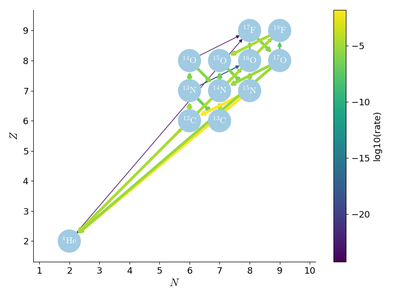
Once the temperature reaches a threshold of \(\gtrsim 10^8\,\mathrm{K}\), the fast \(p\)-captures, for example, \(\isotm{N}{13}(p,\gamma)\isotm{O}{14}\), are more likely than the \(\beta^{+}\)-decays \(\isotm{N}{13}(\beta^{+}\nu_e)\isotm{C}{13}\) reactions. These rates are also included in this network.
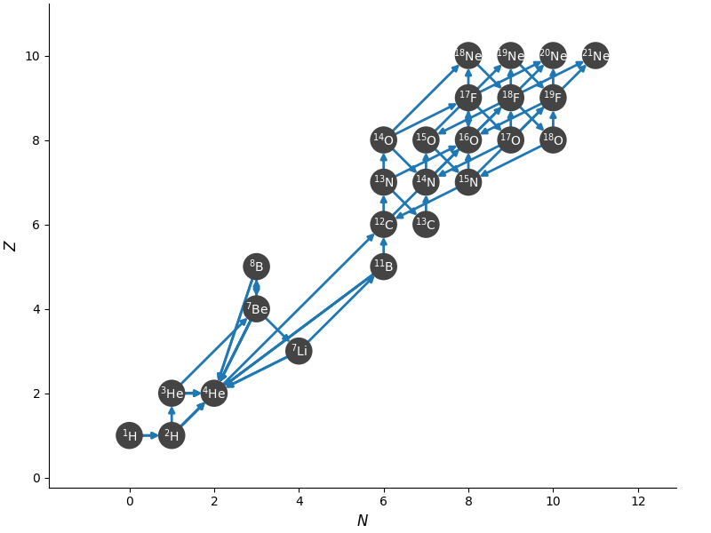
nova-li
This network builds on nova and adds \(\isotm{Li}{7}\) as well as
nuclei beyond fluorine. It should give a more accurate energy in late
stages of the burst, and can also be used to explore lithium
production.
He-burning networks
This is a collection of networks meant to (primarily) model He burning. The are inspired by the “aprox”-family of networks, but contain more nuclei/rates, and are managed by pynucastro.
One feature of these networks is that they include a bypass rate for \(\isotm{C}{12}(\alpha, \gamma)\isotm{O}{16}\) discussed in [22]. This is appropriate for explosive He burning. That paper discusses the sequences:
\(\isotm{C}{14}(\alpha, \gamma)\isotm{O}{18}(\alpha, \gamma)\isotm{Ne}{22}\) at high temperatures (T > 1 GK). We don’t consider this.
\(\isotm{N}{14}(\alpha, \gamma)\isotm{F}{18}(\alpha, p)\isotm{Ne}{21}\) is the one they consider important, since it produces protons that are then available for \(\isotm{C}{12}(p, \gamma)\isotm{N}{13}(\alpha, p)\isotm{O}{16}\).
The problem with this is that it leaves \(\isotm{Ne}{21}\) as an endpoint. We generally do not include it, but instead include approximations to \(\isotm{N}{14}\) from
aprox19, including \(\isotm{N}{14}(1.5\alpha,\gamma)\isotm{Ne}{20}\) proceeding at the rate for \(\isotm{N}{14}(\alpha,\gamma)\isotm{F}{18}\), and \(\isotm{O}{16}(pp,\alpha)\isotm{N}{14}\) proceeding at the rate for \(\isotm{O}{16}(p,\gamma)\isotm{F}{17}\).
For the \(\isotm{C}{12} + \isotm{C}{12}\), \(\isotm{C}{12} + \isotm{O}{16}\), and \(\isotm{O}{16} + \isotm{O}{16}\) rates, we also need to include:
\(\isotm{C}{12}(\isotm{C}{12},n)\isotm{Mg}{23}(n,\gamma)\isotm{Mg}{24}\)
\(\isotm{O}{16}(\isotm{O}{16}, n)\isotm{S}{31}(n, \gamma)\isotm{S}{32}\)
\(\isotm{O}{16}(\isotm{C}{12}, n)\isotm{Si}{27}(n, \gamma)\isotm{Si}{28}\)
Since the neutron captures on those intermediate nuclei are so fast, we leave those out and take the forward rate to just be the first rate. We do not include reverse rates for these processes.
These networks also combine some of the \(A(\alpha,p)X(p,\gamma)B\) links with \(A(\alpha,\gamma)B\), allowing us to drop the intermediate nucleus \(X\). Some will approximate \(A(n,\gamma)X(n,\gamma)B\) into an effective \(A(nn,\gamma)B\) rate (double-neutron capture).
Furthermore, all of these networks rederive the inverse rates from ReacLib using detailed balance and tabulated partition functions.
The networks are named with a descriptive name and the number of nuclei, along with letters:
aif they approximate \((\alpha, p)(p,\gamma)\)mif they include a modified rate that connects odd-Z to even-Z nucleinif they approximate double-neutron capturepif they split the protons into two groups (one for photo-disintegration)
Tip
The alias subch_simple will always point to the smallest of the
He-burning networks (he-burn-*), allowing one to build with
NETWORK_DIR=subch_simple.
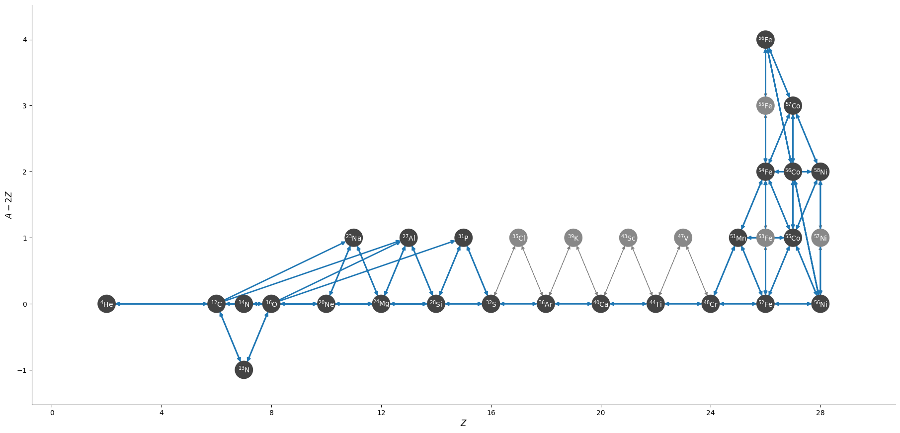
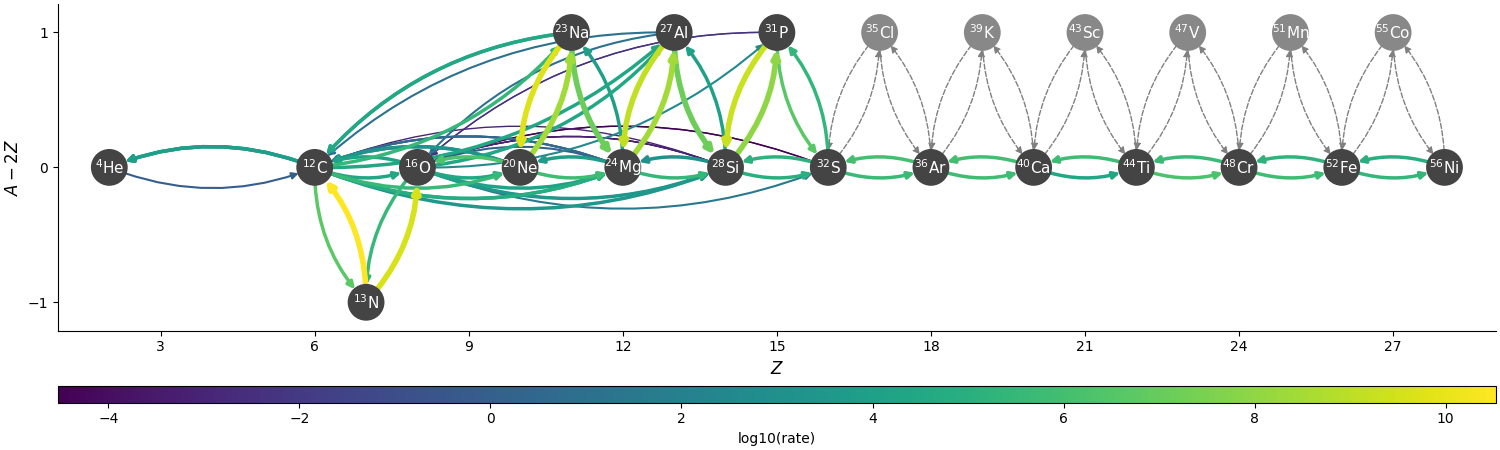
he-burn-19am
This is the simplest network and is similar to aprox13, but includes
a better description of \(\isotm{C}{12}\) and \(\isotm{O}{16}\) burning, as
well as the bypass rate for \(\isotm{C}{12}(\alpha,\gamma)\isotm{O}{16}\).
It has the following features / simplifications:
\(\isotm{Cl}{35}\), \(\isotm{K}{39}\), \(\isotm{Sc}{43}\), \(\isotm{V}{47}\), \(\isotm{Mn}{51}\), and \(\isotm{Co}{55}\) are approximated out of the \((\alpha, p)(p, \gamma)\) links.
The nuclei \(\isotm{N}{14}\) is present with simple links to \(\isotm{Ne}{20}\) and \(\isotm{O}{16}\).
The reverse rates of \(\isotm{C}{12}+\isotm{C}{12}\), \(\isotm{C}{12}+\isotm{O}{16}\), \(\isotm{O}{16}+\isotm{O}{16}\) are neglected since they’re not present in the original aprox13 network
The \(\isotm{C}{12}+\isotm{Ne}{20}\) rate is removed
The \((\alpha, \gamma)\) links between \(\isotm{Na}{23}\), \(\isotm{Al}{27}\) and between \(\isotm{Al}{27}\) and \(\isotm{P}{31}\) are removed, since they’re not in the original aprox13 network.
Overall, there are 19 nuclei and 92 rates.
The network appears as:
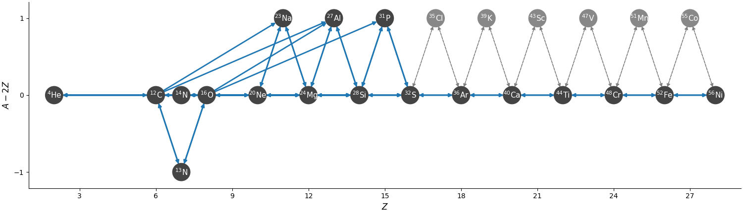
The nuclei in gray are those that have been approximated about, but the links are effectively accounted for in the approximate rates.
There are 2 runtime parameters that can be used to disable rates:
network.disable_p_C12_to_N13_reaclib: if set to1, then the rate \(\isotm{C}{12}(p,\gamma)\isotm{N}{13}\) and its inverse are disabled.network.disable_He4_N13_to_p_O16_reaclib: if set to1, then the rate \(\isotm{N}{13}(\alpha,p)\isotm{O}{16}\) and its inverse are disabled.
Together, these parameters allow us to turn off the sequence \(\isotm{C}{12}(p,\gamma)\isotm{N}{13}(\alpha, p)\isotm{O}{16}\) that acts as a bypass for \(\isotm{C}{12}(\alpha, \gamma)\isotm{O}{16}\).
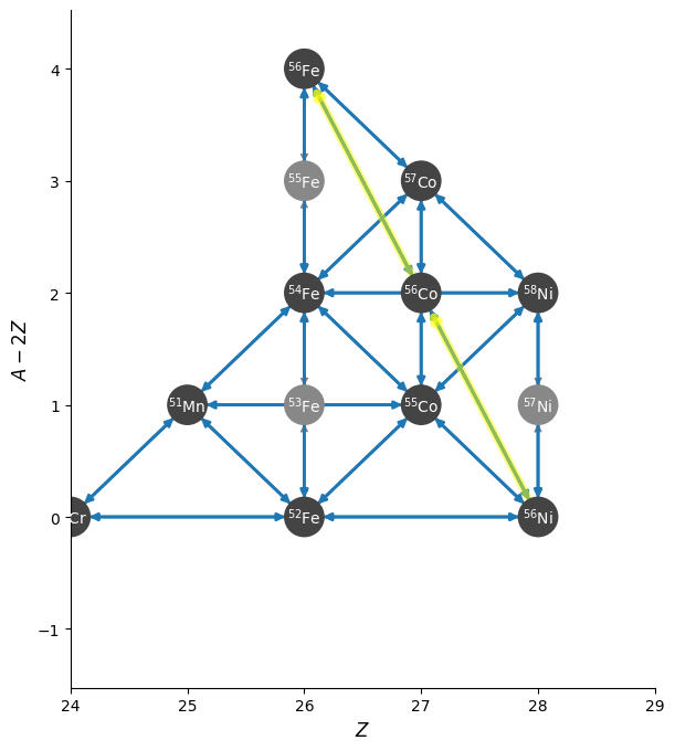
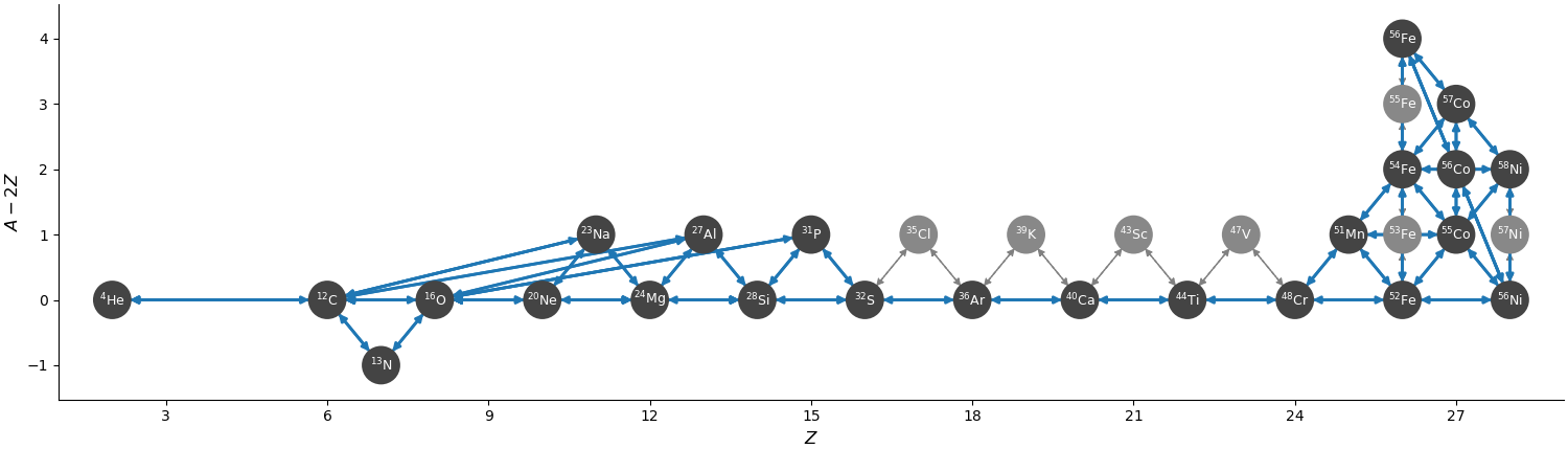
he-burn-28amnp
This builds on he-burn-19am by adding some iron-peak nuclei. It no longer
approximates out \(\isotm{Mn}{51}\) or \(\isotm{Co}{55}\), and includes approximations
to double-neutron capture. Finally, it splits the protons into two groups,
with those participating in reactions with mass numbers > 48 treated as a separate
group (for photo-disintegration reactions).
Overall, there are 28 nuclei and 136 rates, including 6 tabular weak rates.
The iron group here resembles aprox21, but has the addition of stable \(\isotm{Ni}{58}\)
and doesn’t include the approximation to \(\isotm{Cr}{56}\).
The full network appears as:
and a zoom-in on the iron group with the weak rates highlighted appears as:
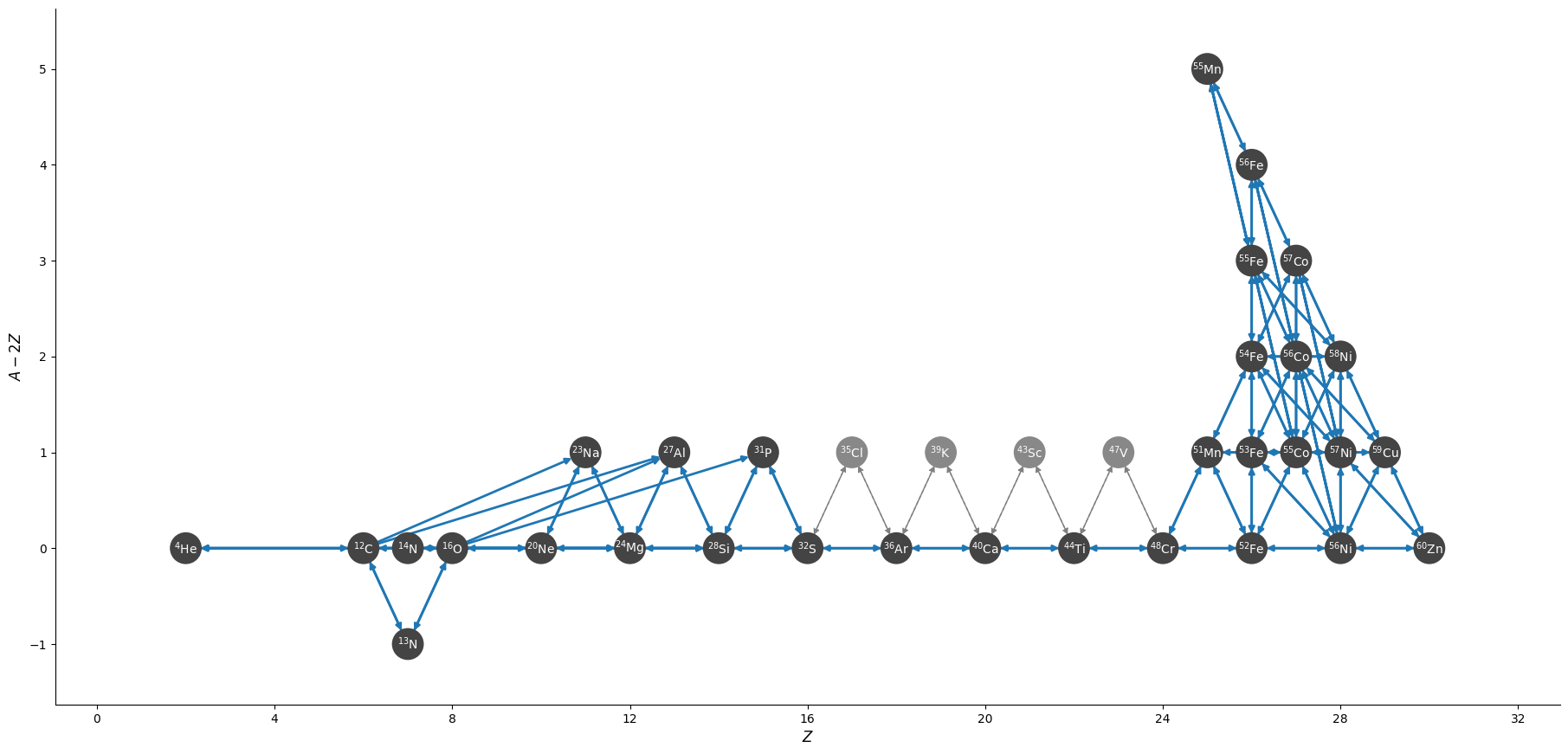
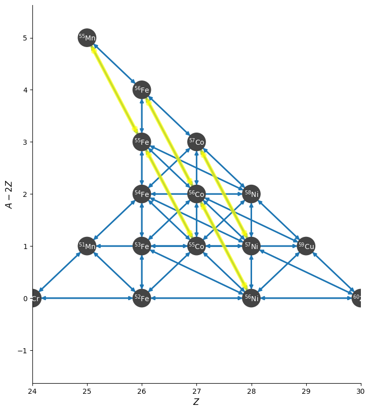
he-burn-33am
This has the most complete iron-group, with nuclei up to \(\isotm{Zn}{60}\) and no approximations to the neutron captures. This network can be quite slow.
Overall, there are 33 nuclei and 172 rates, including 12 tabular weak rates.
The full network appears as:
and a zoom in on the iron group with the weak rates highlighted appears as:
ase
This is a small network like he_burn_19am, but it is carefully
constructed to have reverse rates for all forward rates, allowing
it to be used with the Self-consistent NSE solver. It does not
include \(\isotm{N}{14}\) due to the inability to easily link it to the
\(\alpha\)-chain without a modified rate (which does not behave well with NSE).
The full network appears as:
ase-iron
As with ase, this network is constructed to have reverse rates for all forward rates, allowing
it to be used with the Self-consistent NSE solver. It builds off of ase by including
more iron-group nuclei.
The full network appears as:
Overall there are 28 nuclei with 7 approximated-out nuclei and 153 rates.
cno_he_burn_33a
This network is meant to study explosive H and He burning. It combines
the CNO_extras network (with the exception of the inert \({}^{56}\mathrm{Fe}\)
with the he-burn-19a network. This allows it to capture hot-CNO and
He burning.
Overall there are 33 nuclei and 157 rates, including 10 tabular weak rates.
The network appears as:
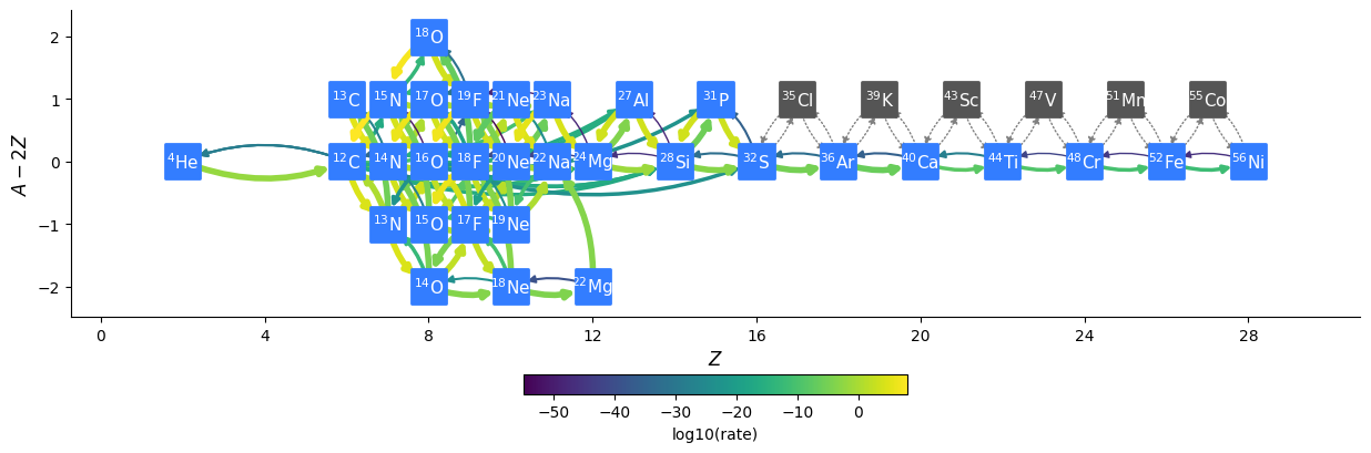
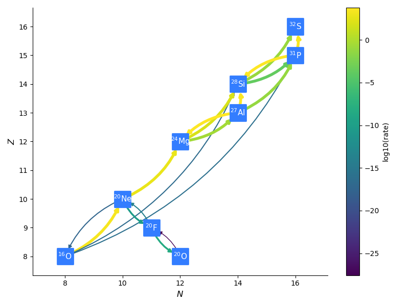
cno_he_burn_34am
This is a better set of nuclei than cno_he_burn_33a that eliminates some
endpoints. It uses an approximate rate to link odd and even nuclei (similar
to how aprox19 and aprox21 connect \(\isotm{N}{14}\).
\(\isotm{Na}{22}(1.5\alpha, \gamma)\isotm{Si}{28}\) is included using the \(\isotm{Na}{22}(\alpha, \gamma)\isotm{Al}{26}\) rate.
\(\isotm{Mg}{24}(pp,\alpha)\isotm{Na}{22}\) is included as an approximation to the sequence \(\isotm{Mg}{24}(p,\gamma)\isotm{Al}{25}(e^+,)\isotm{Mg}{25}(p,\alpha)\isotm{Na}{22}\)
Overall there are 34 nuclei and 179 rates, including 12 tabular weak rates.
The network appears as:
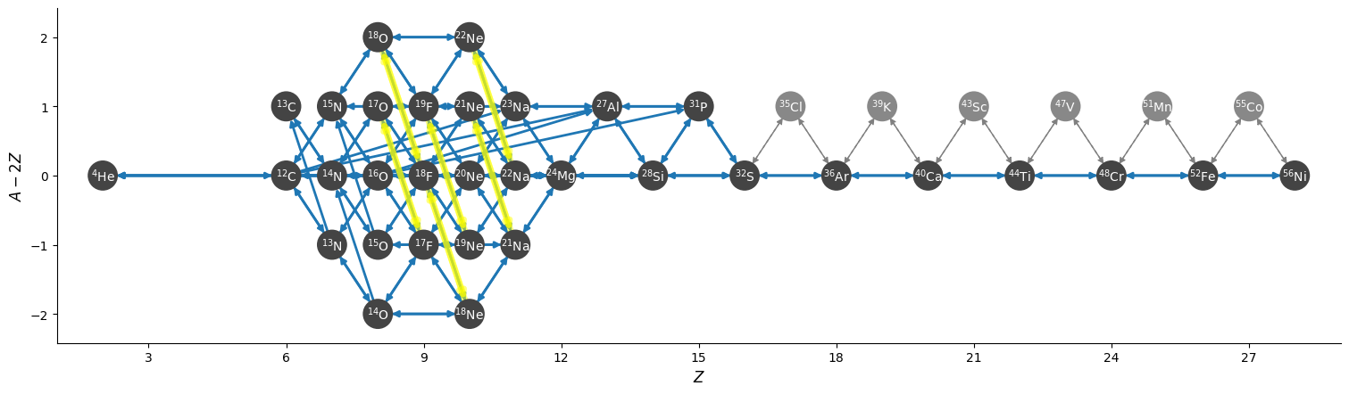
where the tabular rates are highlighted in yellow.
ECSN
ECSN is meant to model electron-capture supernovae in O-Ne white dwarfs.
It includes various weak rates that are important to this process.
C-ignition networks
There are a number of networks that have been developed for exploring carbon burning in near-Chandrasekhar mass which dwarfs.
ignition_chamulak
This network was introduced in our paper on convection in white dwarfs as a model of Type Ia supernovae [23]. It models carbon burning in a regime appropriate for a simmering white dwarf, and captures the effects of a much larger network by setting the ash state and energetics to the values suggested in [24].
The binding energy, \(q\), in this network is interpolated based on the density. It is stored as the binding energy (ergs/g) per nucleon, with a sign convention that binding energies are negative. The energy generation rate is then:
(this is positive since both \(q\) and \(dY/dt\) are negative)
ignition_reaclib
This contains several networks designed to model C burning in WDs. They include:
C-burn-simple: a version ofignition_simplebuilt from ReacLib rates. This just includes the C+C rates and doesn’t group the endpoints together.URCA-simple: a basic network for modeling convective Urca, containing the \({}^{23}\mathrm{Na}\)-\({}^{23}\mathrm{Ne}\) Urca pair.URCA-medium: a more extensive Urca network thanURCA-simple, containing more extensive C burning rates.
ignition_simple
This is the original network used in our white dwarf convection studies [25]. It includes a single-step \(^{12}\mathrm{C}(^{12}\mathrm{C},\gamma)^{24}\mathrm{Mg}\) reaction. The carbon mass fraction equation appears as
where \(N_A \left <\sigma v\right>\) is evaluated using the reaction rate from (Caughlan and Fowler 1988). The Coulomb screening factor, \(f_\mathrm{Coul}\), is evaluated using the general routine from the Kepler stellar evolution code (Weaver 1978), which implements the work of (Graboske 1973) for weak screening and the work of (Alastuey 1978 and Itoh 1979) for strong screening.
powerlaw
This is a simple single-step reaction rate. We will consider only two species, fuel, \(f\), and ash, \(a\), through the reaction: \(f + f \rightarrow a + \gamma\). Baryon conservation requires that \(A_f = A_a/2\), and charge conservation requires that \(Z_f = Z_a/2\). We take our reaction rate to be a powerlaw in temperature. The standard way to write this is in terms of the number densities, in which case we have
with
Here, \(r_0\) sets the overall rate, with units of \([\mathrm{cm^3~s^{-1}}]\), \(T_0\) is a reference temperature scale, and \(\nu\) is the temperature exponent, which will play a role in setting the reaction zone thickness. In terms of mass fractions, \(n_f = \rho X_a / (A_a m_u)\), our rate equation is
We define a new rate constant, \(\rt\) with units of \([\mathrm{s^{-1}}]\) as
where \(\rho_0\) is a reference density and \(T_a\) is an activation temperature, and then our mass fraction equation is:
Finally, for the energy generation, we take our reaction to release a specific energy, \([\mathrm{erg~g^{-1}}]\), of \(\qburn\), and our energy source is
There are a number of parameters we use to control the constants in
this network. This is one of the few networks that was designed
to work with gamma_law as the EOS.
rprox
This network contains 10 species, approximating hot CNO, triple-\(\alpha\), and rp-breakout burning up through \(^{56}\mathrm{Ni}\), using the ideas from [26], but with modern reaction rates from ReacLib [27] where available. This network was used for the X-ray burst studies in [28, 29], and more details are contained in those papers.
triple_alpha_plus_cago
This is a 2 reaction network for helium burning, capturing the \(3\)-\(\alpha\) reaction and \(\isotm{C}{12}(\alpha,\gamma)\isotm{O}{16}\). Additionally, \(^{56}\mathrm{Fe}\) is included as an inert species.