Visualization

Plotfiles

MAESTROeX outputs plotfiles specifically for visualization and analysis. The table below lists the quantities stored in a plotfile. Not all of these may be present, dependent on what options were used in creating the plotfile.

By default, plotfiles store double precision data, but if:

fab.format = NATIVE_32

is set in the inputs file, then the data is converted to single precision before outputting—this is done to reduce file sizes.

Table 3 Plotfile quantities

plotfile variable name	description	runtime parameter controlling output
x_vel	\(\ut\)	–
y_vel	\(\vt\)	–
z_vel	\(\wt\)	3-d runs only
density	\(\rho\)	–
rhoh	\((\rho h)\)	use_tfromp = F or (use_tfromp = T and plot_h_with_use_tfromp = T)
h	\((\rho h)/\rho\)	use_tfromp = F or (use_tfromp = T and plot_h_with_use_tfromp = T)
X(*)	\((\rho X_k)/\rho\)	plot_spec
tracer	tracers	plot_trac
w0_x	\(w_0 \er \cdot \ex\)	plot_base
w0_y	\(w_0 \er \cdot \ey\)	plot_base
w0_z	\(w_0 \er \cdot \ez\)	plot_base
divw0	\(\nabla \cdot w_0\)	plot_base
rho0	\(\rho_0\)	plot_base
rhoh0	\((\rho h)_0\)	plot_base
h0	\((\rho h)_0/\rho_0\)	plot_base
p0	\(p_0\)	plot_base
radial_velocity	\(\Ubt \cdot \er + w_0\)	spherical == 1
circum_velocity	\(|\Ubt - (\Ubt \cdot \er) \er |\)	spherical == 1
magvel	\(| \Ubt + w_0 \er |\)
momentum	\(\rho | \Ubt + w_0 \er |\)
vort	\(| \nabla \times \Ubt |\)
S	\(S\)	–
rhopert	\(\rho - \rho_0\)	–
rhohpert	\((\rho h) - (\rho h)_0\)	use_tfromp = F or (use_tfromp = T and plot_h_with_use_tfromp = T)
tfromp	\(T(\rho, p_0, X_k)\)	–
tfromh	\(T(\rho, h, X_k)\)	use_tfromp = F or (use_tfromp = T and plot_h_with_use_tfromp = T)
deltaT	\([T(\rho, h, X_k) -\) \(T(\rho, p_0, X_k)]\) \(/T(\rho, h, X_k)\)	use_tfromp = F or (use_tfromp = T and plot_h_with_use_tfromp = T)
deltap	\(|p(\rho,h,X_k)-p_0|/p_0\)	use_tfromp = F or (use_tfromp = T and plot_h_with_use_tfromp = T)
tpert	\(T(\rho,h,X_k)-\overline{T}\) if use_tfromp = F; \(T(\rho,p_0,X_k)-\overline{T}\) otherwise	–
Machnumber	\(|\Ubt+w_0\er |/c(\rho,p_0,X_k)\)	–
soundspeed	\(c(\rho,p_0,X_k)\)	plot_cs
deltagamma	\(\Gamma_1-\gammabar\)	–
entropy	\(s(\rho,p_0,X_k)\)	–
entropypert	\([s(\rho,p_0,X_k) -\) \(\overline{s}]/\overline{s}\)	–
sponge or sponge_fdamp	\(1/(1+\Delta t\kappa \fdamp)\) by default; \(\fdamp\) if plot_sponge_fdamp = T	–
pi	\(\pi\)	–
gpi_x	\(\nabla \pi \cdot \ex\)	plot_gpi
gpi_y	\(\nabla \pi \cdot \ey\)	plot_gpi
gpi_z	\(\nabla \pi \cdot \ez\)	plot_gpi
pioverp0	\(\pi / p_0\)	plot_base
p0pluspi	\(p_0 + \pi\)	plot_base
omegadot(*)	\(\dot{\omega}_k\)	plot_omegadot
enucdot	\((\rho \Hnuc)/\rho\)	plot_Hnuc
Hext	\((\rho \Hext)/\rho\)	plot_Hext
eta_rho	\(\etarho\)	plot_eta
thermal	\(\nabla \cdot \kappa\nabla T\)	use_thermal_diffusion
conductivity	\(\kappa(\rho, T,X_k)\)	use_thermal_diffusion
ad_excess	\(\nabla - \nabla_\mathrm{ad}\)	plot_ad_excess
particle_count	number of particles in a cell	use_particles
processor_number	processor number containing the cell’s data	plot_processors
pi_divu	\(\pi \nabla \cdot\tilde{\Ub}\) (a measure of energy conservation)	plot_pidivu

Small vs. regular plotfiles

MAESTROeX can manage two independent sets of plotfiles. This allows you to output the default plotfiles, which contain a lot of variables, sparsely, and output small-plotfiles much more frequently. A small-plotfile is controlled by the analogous runtime parameters as the main plotfiles:

• small_plot_int is the interval in steps between successive plotfiles

• small_plot_deltat is the interval in time between successive plotfiles

• small_plot_base_name is the base name that prefixes the plotfiles. The default is smallplt

The fields that are stored in the small plotfiles is set by the runtime parameter small_plot_vars. This should be a (space-separated) list of the parameter names to be included in the plot file.

Visualizing with Amrvis

Amrvis is a tool developed together with AMReX to visualize datasets from codes built around the AMReX library. To download and build Amrvis, follow the instructions in the AMReX documentation: https://amrex-codes.github.io/amrex/docs_html/Visualization.html

Once the code is built, you visualize a dataset as:

amrvis3d.Linux.g++.gfortran.ex pltfile

where pltfile is the name of the plotfile directory. Different variables can be selected from the drop down menu at the top. Middle and right clicking in 3-d select the slice planes, and shift + middle or right will extract 1-d lines through the data. In 2-d, middle and right clicking alone extract 1-d lines.

If Amrvis cannot find the Palette file, then the plots will be in grayscale. To fix this, copy the amrvis.defaults and Palette files to your home directory and edit amrvis.defaults so that the palette line points to the Palette file, e.g.:

palette               /home/username/Palette

Visualizing with VisIt

VisIt recognizes MAESTROeX plotfiles as being in the BoxLib format.

Visualizing with yt

yt is a Python package for analyzing and visualizing simulation data, and understand that AMReX data from MAESTROeX and CASTRO (along with many other simulation codes). For more information, see the yt homepage at http://yt-project.org/ and [TurkSmithOishi+11].

Some sample scripts that use yt with MAESTROeX data are contained in MAESTROeX/Util/yt/.

plotsinglevar.py

plotsinglevar.py does visualizations of 2-d AMReX plotfiles, and slices through 3-d AMReX plotfiles. A simple plot can be made via:

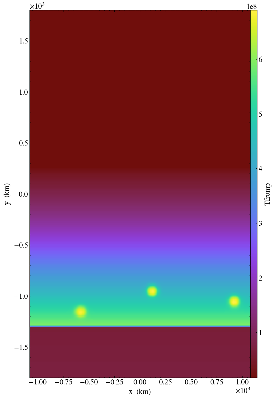
python plotsinglevar.py --log -o test.png plt00000/ tfromp

This will make a plot of “tfromp” from the plotfile plt00000 with log scaling, and store the output in test.png, as showing the figure below. If you don’t do ‘-o’, then a default output filename consisting of the plotfile name + component will be used.

Fig. 14 Plot of reacting_bubble done with the python script plotsinglevar.py.

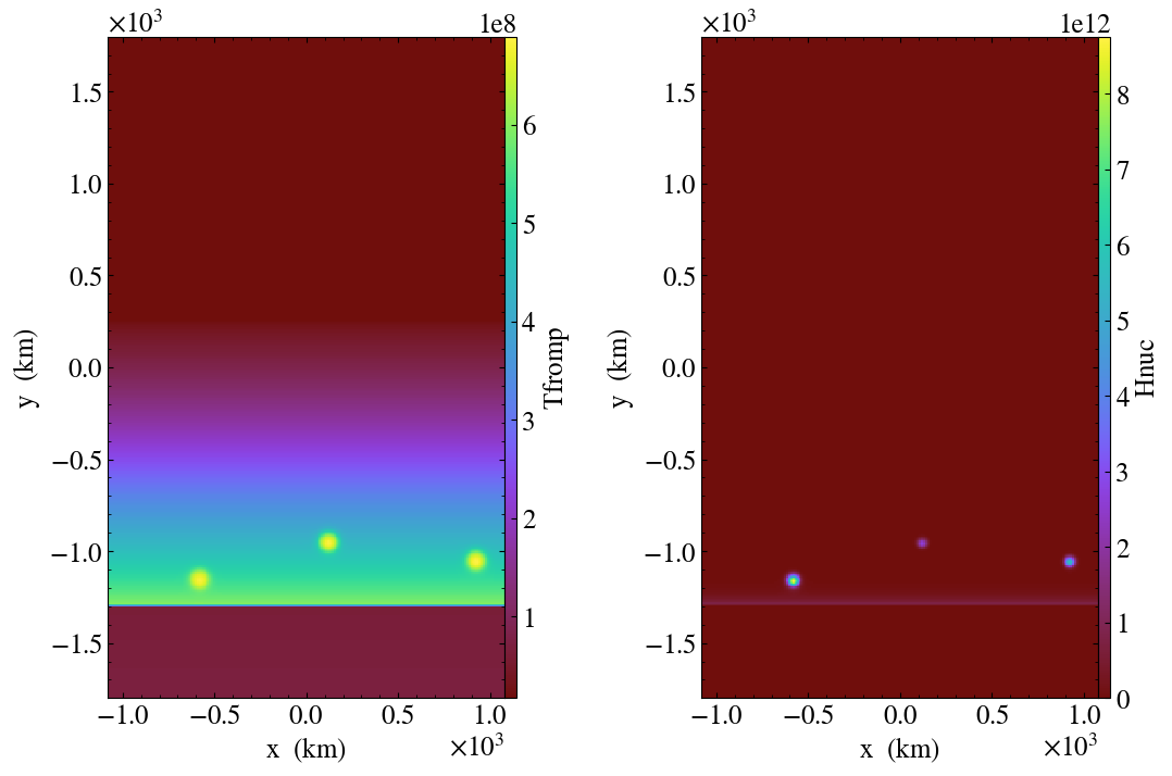
If you list 2 different variables after the plotfile name, then they will be plotted side-by-side in a single figure. For example,

python plotsinglevar.py plt00000/ tfromp Hnuc

produces the output shown below:

Fig. 15 Plot of reacting_bubble done with the python script plotsinglevar.py showing 2 variables plotted from a single plotfile.

Additional options include ‘-min’ to specify the minimum data value, and ‘-max’ to specify the maximum data value. Running the script with the flag -h will list the available options.

3-d support is available. When run as with a plotfile name and variable, it will plot slices (\(x\)-\(y\), \(x\)-\(z\), and \(y\)-\(z\)) through the center of the domain.

contourcompare.py

contourcompare.py takes two or three plotfiles and a single variable as arguments and plots contours of the datasets on the same set of axes. This is facilitates comparisons of different runs. Running the script with the flag -h will give the full list of available options.

For example:

python contourcompare.py tfromp plt00000 other_plt00000

will make a contour plot of the variable tfromp from the data in plt00000 and other_plt00000 shown on the same axes.

runtimevis.py

The runtimevis.py script is designed to be run from a submission script to produce plots from plotfiles as they are produced.

The script itself reads in an inputs file, vis.in, that describes the variables to plot. From 1 to 6 variables can be plotting from a plotfile. The script does its best to organize them in columns and rows to maximize the plot area. The image is always output at 1280\(\times\)720 pixels, corresponding to 720p HD resolution. For each variable, a block of the form:

[varname]
min = 1
max = 2
log = 1

is supplied. If min or max are omitted, then the data limits are computed automatically. If log is omitted, then no log is taken of the data before plotting. The script is then run as:

python runtimevis.py plt00000