`burn_cell`

burn_cell is a simple one-zone burn that will evolve a state with a network for a specified amount of time. This can be used to understand the timescales involved in a reaction sequence or to determine the needed ODE tolerances. This is designed to work with the Strang-split integration wrappers. The system that is evolved has the form:

\begin{array}{r} \begin{aligned} \frac{d X_{k}}{d t} & = {\dot{ω}}_{k} (ρ, X_{k}, T) \\ \frac{d e}{d t} & = ϵ (ρ, X_{k}, T) \end{aligned} \end{array}

with density held constant and the temperature found via the equation of state, $T = T (ρ, X_{k}, e)$ .

Note

Since the energy evolves due to the heat release (or loss) from reactions, the temperature will change during the burn (unless integrator.call_eos_in_rhs=0 is set).

Getting Started

The burn_cell code is located in Microphysics/unit_test/burn_cell. An inputs file which sets the default parameters for your choice of network is needed to run the test. There are a number of inputs files in the unit test directory already with a name list inputs_network, where network is the network you wish to use for your testing. These can be used as a starting point for any explorations.

Setting the thermodynamics

The parameters that affect the thermodynamics are:

unit_test.density : the initial density
unit_test.temperature : the initial temperature

The composition can be set either by specifying individual mass fractions or setting unit_test.uniform_xn as described in Defining composition.

If the values don’t sum to 1 initially, then the test will do a normalization. This normalization can be disabled by setting:

unit_test.skip_initial_normalization = 1

Controlling time

The test will run unit a time unit_test.tmax, outputting the state at regular intervals. The parameters controlling the output are:

unit_test.tmax : the end point of integration.
unit_test.tfirst : the first time interval to output.
unit_test.nsteps : the number of steps to divide the integration into, logarithmically-spaced.

If there is only a single step, unit_test.nsteps = 1, then we integrate from $[0, tmax]$ .

If there are multiple steps, then the first output will be at a time $tmax / nsteps$ , and the steps will be logarithmically-spaced afterwards.

Integration parameters

The tolerances, choice of Jacobian, and other integration parameters can be set via the usual Microphysics runtime parameters, e.g. integrator.atol_spec.

Building and Running the Code

The code can be built simply as:

make

and the network and integrator can be changed using the normal Microphysics build system parameters, e.g.,

make NETWORK_DIR=aprox19 INTEGRATOR_DIR=rkc

The build process will automatically create links in the build directory to the EOS table and any reaction rate tables needed by your choice of network.

Important

You need to do a make clean before rebuilding with a different network or integrator.

To run the code, in the burn_cell directory run:

./main3d.gnu.ex inputs

where inputs is the name of your inputs file.

Working with Output

Note

For this part, we’ll assume that the default aprox13 and VODE options were used for the network and integrator, and the test was run with inputs.aprox13.

As the code runs, it will output to stdout details of the initial and final state and the number of integration steps taken (along with whether the burn was successful). The full history of the thermodynamic state will also be output to a file, state_over_time.txt, with each line corresponding to one of the nsteps requested in the time integration.

The script plot_burn_cell.py can be used to visualize the evolution:

python plot_burn_cell.py state_over_time.txt

This will generate the following figure:

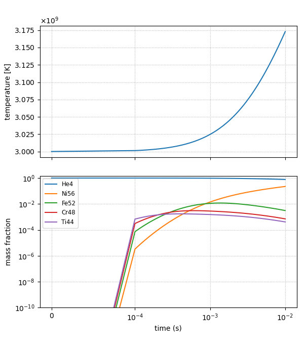
An example of a plot output by the burn_cell unit test.

Only the most abundant species are plotted. The number of species to plot and the limits of $X$ can be set via runtime parameters (see python plot_burn_cell.py -h).

burn_cell