Verification
Hydrodynamics Test Problems
Sod’s Problem (and Other Shock Tube Problems)
The Exec/hydro_tests/Sod problem directory sets up a general one-dimensional shock tube. The left and right primitive-variable states are specified and the solution evolves until a user-specified end time. For a simple discontinuity, the exact solution can be found from an exact Riemann solver. For this problem, the exact solutions were computed with the exact Riemann solver from Toro [14], Chapter 4.
Sod’s Problem
The Sod problem [64] is a simple shock tube problem that exhibits a shock, contact discontinuity, and a rarefaction wave. The initial conditions are:
The gamma_law equation of state is used with \(\gamma = 1.4\). The system is evolved until \(t = 0.2\) s. Setups for 1-, 2-, and 3-d are provided. The following inputs files setup the Sod’s problem:
|
Sod’s problem along \(x\)-direction |
|
Sod’s problem along \(y\)-direction |
|
Sod’s problem along \(z\)-direction |
For multi-dimensional runs, the directions transverse to the jump are kept constant. We use a CFL number of 0.9, an initial timestep shrink (castro.init_shrink) of 0.1, and the maximum factor by which the timestep can increase (castro.change_max) of 1.05.
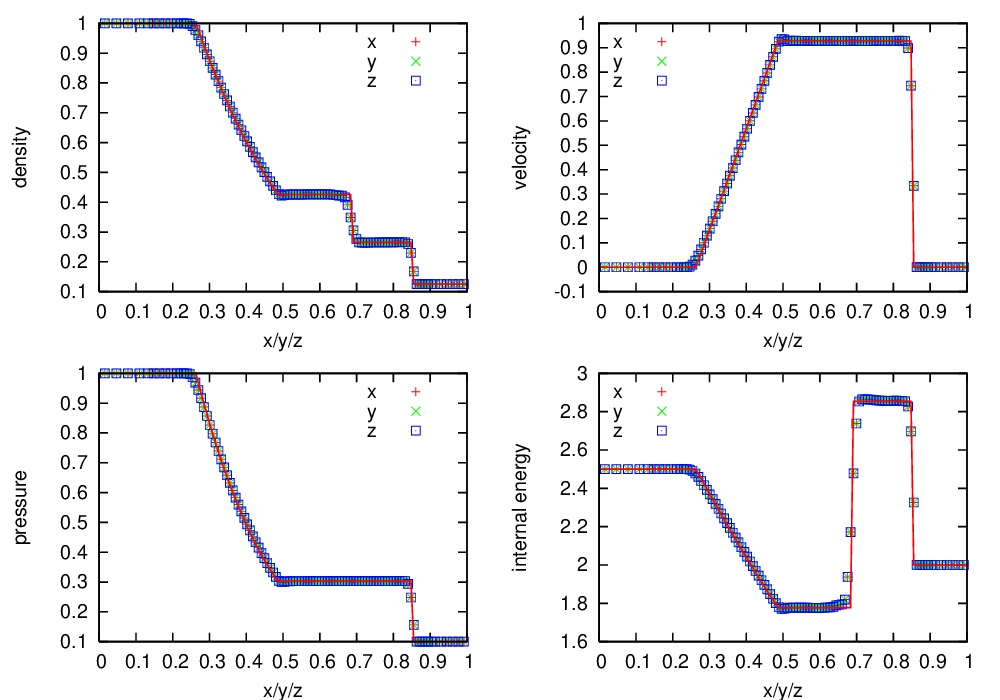
Fig. 10 Castro solution for Sod’s problem run in 3-d, with the newest ppm limiters, along the \(x\), \(y\), and \(z\) axes. A coarse grid of 32 zones in the direction of propagation, with 2 levels of refinement was used. The analytic solution appears as the red line.
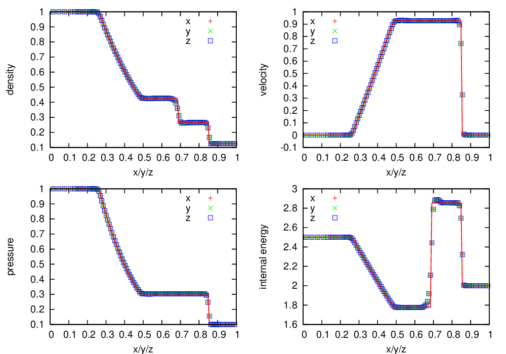
Fig. 11 Castro solution for Sod’s problem run in 3-d, with the piecewise-linear Godunov method with limiters, along the \(x\), \(y\), and \(z\) axes. A coarse grid of 32 zones in the direction of propagation, with 2 levels of refinement was used. The analytic solution appears as the red line.
Fig. 10 shows the Castro solution using the newest PPM limiters compared to the analytic solution, showing the density, velocity, pressure, and internal energy. Fig. 11 is the same as Fig. 10, but with the piecewise-linear Godunov method with limiters, shown for comparison.
The Verification subdirectory includes the analytic solution for
the Sod problem sod-exact.out, with \(\gamma = 1.4\). 1-d slices
can be extracted from the Castro plotfile using the fextract tool
from amrex/Tools/Postprocessing/C_Src/.
The steps to generate this verification plot with Castro are:
in
Exec/hydro_tests/Sod, build the Castro executable in 3-drun the Sod problem with Castro in the \(x\), \(y\), and \(z\) directions:
./Castro3d.Linux.Intel.Intel.ex inputs-sod-x
./Castro3d.Linux.Intel.Intel.ex inputs-sod-y
./Castro3d.Linux.Intel.Intel.ex inputs-sod-z
build the fextract tool in
amrex/Tools/Postprocessing/C_Src/.run fextract on the Castro output to generate 1-d slices through the output:
fextract3d.Linux.Intel.exe -d 1 -s sodx.out -p sod_x_plt00034
fextract3d.Linux.Intel.exe -d 2 -s sody.out -p sod_y_plt00034
fextract3d.Linux.Intel.exe -d 3 -s sodz.out -p sod_z_plt00034
copy the sodx/y/z.out files into the
Verification/directory.in
Verification/run the gnuplot scriptsod_3d.gpas:gnuplot sod_3d.gp
This will produce the figure
sod_3d.eps.
Double Rarefaction
The double rarefaction is the “Test 2” problem described by Toro [14], Chapter 6. In this test, the center of the domain is evacuated as two rarefaction waves propagate in each direction, outward from the center. It is difficult to get the internal energy to behave at the center of the domain because we are creating a vacuum. The initial conditions are:
The gamma_law equation of state is used with \(\gamma = 1.4\). The system is evolved until \(t = 0.15\) s. Setups for 1-, 2-, and 3-d are provided. The following inputs files setup the double rarefaction problem:
|
Double rarefaction problem along \(x\)-direction |
|
Double rarefaction problem along \(y\)-direction |
|
Double rarefaction problem along \(z\)-direction |
We use a CFL number of 0.8, an initial timestep shrink
(castro.init_shrink) of 0.1, and the maximum factor by which the
timestep can increase (castro.change_max) of 1.05. The PPM solver with
the new limiters are used.
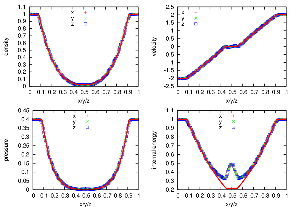
Fig. 12 Castro solution for the double rarefaction problem run in 3-d, along the \(x\), \(y\), and \(z\) axes. A coarse grid of 32 zones in the direction of propagation, with 2 levels of refinement was used. The analytic solution appears as the red line.
Fig. 12 shows the Castro output, run along all 3 coordinate axes in 3-d, compared to the analytic solution.
The comparison to the analytic solution follows the same procedure as
described for the Sod’s problem above. The gnuplot script
test2_3d.gp will generate the figure, from the 1-d slices created by
fextract named test2x.out, test2y.out, and test2z.out.
Strong Shock
The strong shock test is the “Test 3” problem described by Toro [14], Chapter 6. In this test, a large pressure jump at the initial interface creates a very strong rightward moving shock, followed very closely by a contact discontinuity. The initial conditions are:
The gamma_law equation of state is used with \(\gamma = 1.4\). The system is evolved until \(t = 0.012\) s. Setups for 1-, 2-, and 3-d are provided. The following inputs files and probin files setup the strong shock problem:
|
Strong shock problem along \(x\)-direction |
|
Strong shock problem along \(y\)-direction |
|
Strong shock problem along \(z\)-direction |
We use a CFL number of 0.9, an initial
timestep shrink (castro.init_shrink) of 0.1, and the maximum factor by which
the timestep can increase (castro.change_max) of 1.05. The PPM
solver with the new limiters are used.
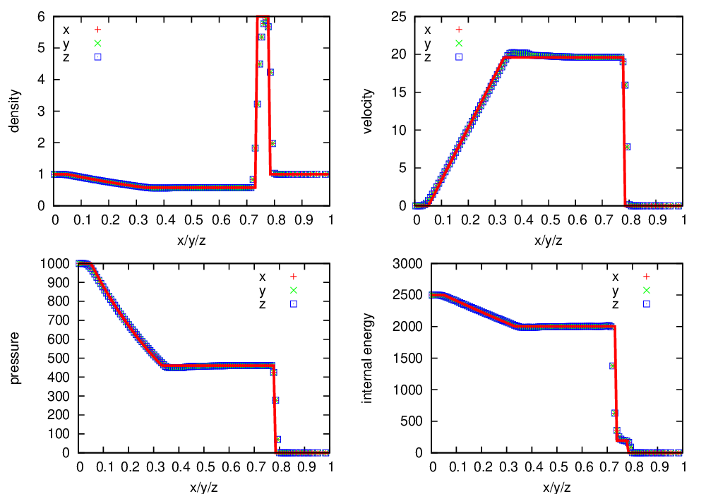
Fig. 13 Castro solution for the strong shock problem run in 3-d, along the \(x\), \(y\), and \(z\) axes. A coarse grid of 32 zones in the direction of propagation, with 2 levels of refinement was used. The analytic solution appears as the red line.
Fig. 13 shows the Castro output, run along all 3 coordinate axes in 3-d, compared to the analytic solution.
The comparison to the analytic solution follows the same procedure as
described for the Sod’s problem above. The gnuplot script
test3_3d.gp will generate the figure, from the 1-d slices created by
fextract named test3x.out, test3y.out, and test3z.out.
Sedov Problem
The Sedov (or Sedov-Taylor) blast wave is a standard hydrodynamics test problem. A large amount of energy is placed into a very small volume, driving a spherical or cylindrical blast wave. Analytic solutions were found by Sedov [63].
A cylindrical blast wave (e.g. a point explosion in a 2-d plane) can
be modeled in 1-d cylindrical coordinate or 2-d Cartesian coordinates.
A spherical blast wave can be modeled in 1-d spherical, 2-d axisymmetric
(cylindrical \(r\)-\(z\)), 2-d axisymmetric
(spherical \(r\)-\(\theta\)),or 3-d Cartesian coordinates.
This provides a good test on the geometric factors in the hydrodynamics solver.
We use a publicly available code, sedov3.f
[49], to generate the analytic solutions.
The Castro implementation of the Sedov problem is in
Exec/hydro_tests/Sedov/. A number of different inputs files
are provided, corresponding to different Sedov/Castro geometries. The
main ones are:
inputs file |
description |
|---|---|
|
Spherical Sedov explosion modeled in 1-d cylindrical coordinates |
|
Spherical Sedov explosion modeled in 1-d spherical coordinates |
|
Spherical Sedov explosion modeled in 2-d cylindrical (axisymmetric) coordinates. |
|
Spherical Sedov explosion modeled in 2-d spherical (axisymmetric) coordinates. |
|
Cylindrical Sedov explosion modeled in 2-d Cartesian coordinates. |
|
Spherical Sedov explosion modeled in 3-d Cartesian coordinates. |
In the Sedov problem, the explosion energy, \(E_\mathrm{exp}\) (in units of energy, not energy/mass or energy/volume) is to be deposited into a single point, in a medium of uniform ambient density, \(\rho_\mathrm{ambient}\), and pressure, \(p_\mathrm{ambient}\). Initializing the problem can be difficult because the small volume is typically only a cell in extent. This can lead to grid imprinting in the solution. A standard solution (see for example [60] and the references therein) is to convert the explosion energy into a pressure contained within a certain volume, \(V_\mathrm{init}\), of radius \(r_\mathrm{init}\) as
This pressure is then deposited in all of the cells where \(r < r_\mathrm{init}\).
To further minimize any grid effects, we do subsampling in each zone: each zone is divided it into \(N_\mathrm{sub}\) subzones in each coordinate direction, each subzone is initialized independently, and then the subzones are averaged together (using a volume weighting for spherical or cylindrical/axisymmetric Castro grids) to determine the initial state of the full zone.
For these runs, we use \(\rho_\mathrm{ambient} = 1\), \(p_\mathrm{ambient} = 10^{-5}\), \(E_\mathrm{exp} = 1\), \(r_\mathrm{init} = 0.01\), and \(N_\mathrm{sub} = 10\). A base grid with 32 zones in each coordinate direction plus 3 levels of refinement is used (the finest mesh would correspond to 256 zones in a coordinate direction). The domain runs from 0 to 1 in each coordinate direction.
An analysis routines for the Sedov problem is provided in
Castro/Diagnostics/Sedov/. Typing make should build it (you
can specify the dimensionality with the DIM variable in the
build).
A spherical Sedov explosion can be modeled in 1-d spherical, 2-d cylindrical (axisymmetric), 2-d spherical (axisymmetric), or 3-d Cartesian coordinates, using the inputs files described in Table 10. A 1-d radial profile can be extracted using the analysis routine. For example, to run and process the 2-d spherical Sedov explosion in cylindrical coordinates, one would do:
in
Exec/hydro_tests/Sedov, build the Castro executable in 2-d:make DIM=2
run the spherical Sedov problem with Castro in 2-d cylindrical coordinates:
./Castro2d.gnu.MPI.ex inputs.2d.sph_in_cylcoords
build the
sedov_2d.extool inCastro/Diagnostics/Sedov:make DIM=2
run the analysis script on the Castro output to generate 1-d radial profiles:
./sedov_2d.ex -s sedov_2d_sph_in_cyl.out \
     -p ../sedov_2d_sph_in_cyl_plt00130
A similar procedure can be used for the spherical and cylindrical
Sedov explosions in other geometries and dimensions. Once this is done,
the sedov_sph.gp and sedov_cyl.gp gnuplot script can be used to
make a plot comparing the numerical solutions to the analytic solution
for spherical and cylindrical Sedov explosions, which are contained
in spherical_sedov.dat and cylindrical_sedov.dat, respectively.
Note that the file containing the 1-d radial profiles of the numerical
solution has the same name as the one specified in the gnuplot script.
- Fig. 14 shows the comparison of the 3 Castro spherical
Sedov explosion simulations to the analytic solution.
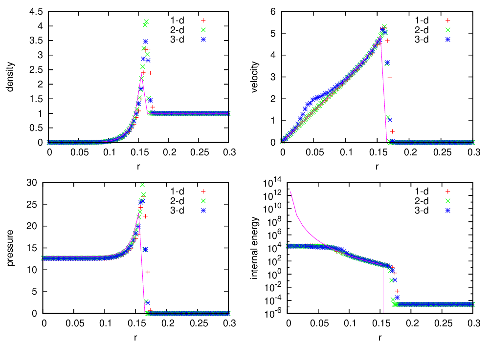
Fig. 14 Castro solution for the Sedov blast wave problem run in 1-d spherical, 2-d cylindrical, 2-d spherical, and 3-d Cartesian coordinates. Each of these geometries produces a spherical Sedov explosion.
Cylindrical Blast Wave
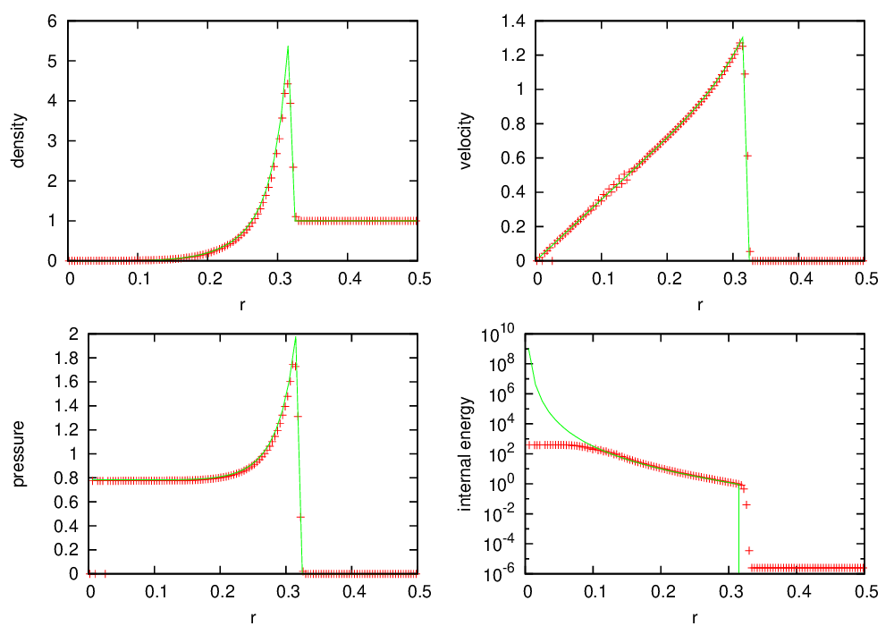
Fig. 15 Castro solution for the Sedov blast wave problem run in 1-d cylindrical and 2-d Cartesian coordinates. This corresponds to a cylindrical Sedov explosion.
Rayleigh-Taylor
2D. Domain size 0.5 by 1.0. 256 by 512 cells, single level calculation. Periodic in x, solid walls on top and bottom in y. Gamma law gas with \(\gamma=1.4\), no reactions. Zero initial velocity. Constant \(|\gb|=1\). The density profile is essentially \(\rho=1\) on bottom, \(\rho=2\) on top, but with a perturbation. A single-mode perturbation is constructed as:
We note that the symmetric form of the cosine is done to ensure that roundoff error does not introduce a left-right asymmetry in the problem. Without this construction, the R-T instability will lose its symmetry as it evolves. This then applied to the interface with a tanh profile to smooth the transition between the high and low density material:
Hydrostatic pressure with \(p=5.0\) at bottom of domain, assuming \(\rho=1\) on the lower half of the domain, and \(\rho=2\) on the upper half and no density perturbation. We run to \(t=2.5\) with piecewise linear, old PPM, and new PPM. CFL=0.9. See Fig. 16.
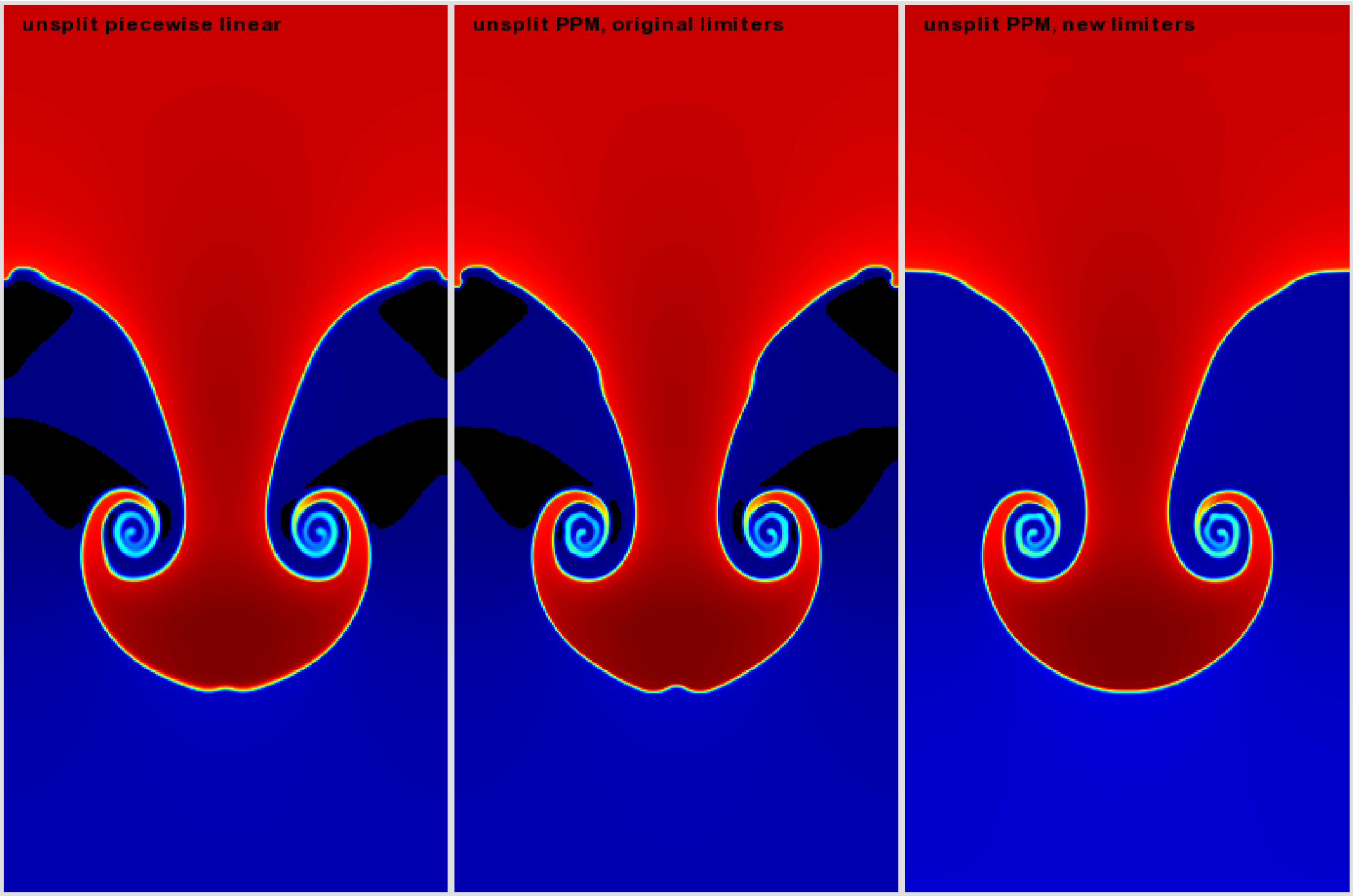
Fig. 16 Rayleigh-Taylor with different PPM types.
Gravity Test Problems
Radiation Test Problems
There are two photon radiation solvers in Castro—a gray solver and a multigroup solver. The gray solver follows the algorithm outlined in [45]. We use the notation described in that paper. In particular, the radiation energy equation takes the form of:
Here, \(E_R\) is the radiation energy density, \(\kappa_R\) is the Roseland-mean opacity, \(\kappa_P\) is the Planck-mean opaciy, and \(\lambda\) is a quantity \(\le 1/3\) that is subjected to limiting to keep the radiation field causal. Castro allows for \(\kappa_R\) and \(\kappa_P\) to be set independently as power-laws.
Light Front
The light front problem tests the ability of the radiation solver to operate in the free-streaming limit. A radiation front is established by initializing one end of the computational domain with a finite radiation field, and zero radiation field everywhere else. The speed of propagation of the radiation front is keep in check by the flux-limiters, to prevent it from exceeding \(c\).
Diffusion of a Gaussian Pulse
The diffusion of a Gaussian pulse problem tests the diffusion term in the radiation energy equation. The radiation energy density is initialized at time \(t = t_0\) to a Gaussian distribution:
As the radiation diffuses, the overall distribution will remain Gaussian, with the time-dependent solution of:
Radiation Source Problem
The radiation source problem tests the coupling between the radiation field and the gas energy through the radiation source term. The problem begins with the radiation field and gas temperature out of equilibrium. If the gas is too cool, then the radiation field will heat it. If the gas is too hot, then it will radiate and cool. In each case, the gas energy and radiation field will evolve until thermal equilibrium is achieved.
Our implementation of this problem follows that of [67].
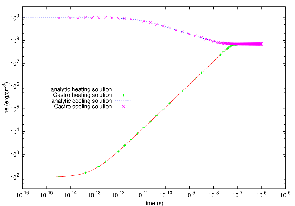
Fig. 17 Castro solution for radiating source test problem. Heating and cooling solutions are shown as a function of time, compared to the analytic solution. The gray photon solver was used.
Radiating Sphere
The radiating sphere (RadSphere) is a multigroup radiation test problem. A hot sphere is centered at the origin in a spherical geometry. The spectrum from this sphere follows a Planck distribution. The ambient medium is at a much lower temperature. A frequency-dependent opacity makes the domain optically thin for high frequencies and optically thick for low frequency. At long times, the solution will be a combination of the blackbody radiation from the ambient medium plus the radiation that propagated from the hot sphere. An analytic solution exists [42] which gives the radiation energy as a function of energy group at a specified time and distance from the radiating sphere.
Our implementation of this problem is in Exec/radiation_tests/RadSphere and follows that of [67]. The routine that computes the analytic solution is provided as analytic.f90.
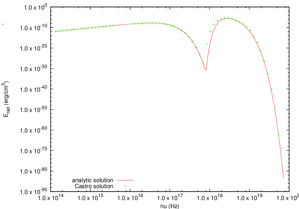
Fig. 18 Castro solution for radiating sphere problem, showing the radiation energy density as a function of energy group. This test was run with 64 photon energy groups.
Regression Testing
An automated regression test suite for Castro (or any AMReX-based code) written in Python exists in the AMReX-Codes github organization.