Rotation

Introduction

Currently, Castro supports constant, solid-body rotation about a fixed (in space and time) axis in 2D and 3D by transforming the evolution equations to the rotating frame of reference.

To include rotation you must set:

USE_ROTATION = TRUE

in the GNUMakefile. Rotation can then be enabled via:

castro.do_rotation = 1

in the inputs file. The rotational period must then be set via castro.rotational_period. The rotational period is internally converted to an angular frequency for use in the source term equations.

The axis of rotation currently depends on the dimensionality of the problem and the value of coord_sys; in all cases, however, the default axis of rotation points from problem::center in the vertical direction.

Note

make sure you have set the problem::center() variable appropriately for you problem. This can be done by directly setting it in the problem_initialize() function.

The “vertical direction” is defined as follows:

• 2D

  • coord_sys = 0, (x,y): out of the (x,y)-plane along the “z”-axis

  • coord_sys = 1, (r,z): along the z-axis

• 3D

  • coord_sys = 0, (x,y,z): along the z-axis

To change these defaults, modify the omega vector in the ca_rotate routine found in the Rotate_$(DIM)d.f90 file.

The main parameters that affect rotation are:

• castro.do_rotation : include rotation as a forcing term (0 or 1; default: 0)

• castro.rotational_period : period (s) of rotation (default: 0.0)

• castro.rotational_dPdt : d(period) / dt for rotation (default: 0.0)

• castro.rotation_include_centrifugal : whether to include the centrifugal forcing (default: 1)

• castro.rotation_include_coriolis : whether to include the Coriolis forcing (default: 1)

• castro.rotation_include_domegadt : whether to include the forcing from the time derivative of the rotation frequency (default: 1)

• castro.rot_source_type : method of updating the energy during a rotation update (default: 4)

• castro.implicit_rotation_update : for the Coriolis term, which mixes momenta in the source term, whether we should solve for the update implicitly (default: 1)

• castro.rot_axis : rotation axis (default: 3 (Cartesian); 2 (cylindrical))

For completeness, we show below a derivation of the source terms that appear in the momentum and total energy evolution equations upon switching to a rotating reference frame.

Coordinate transformation to rotating frame

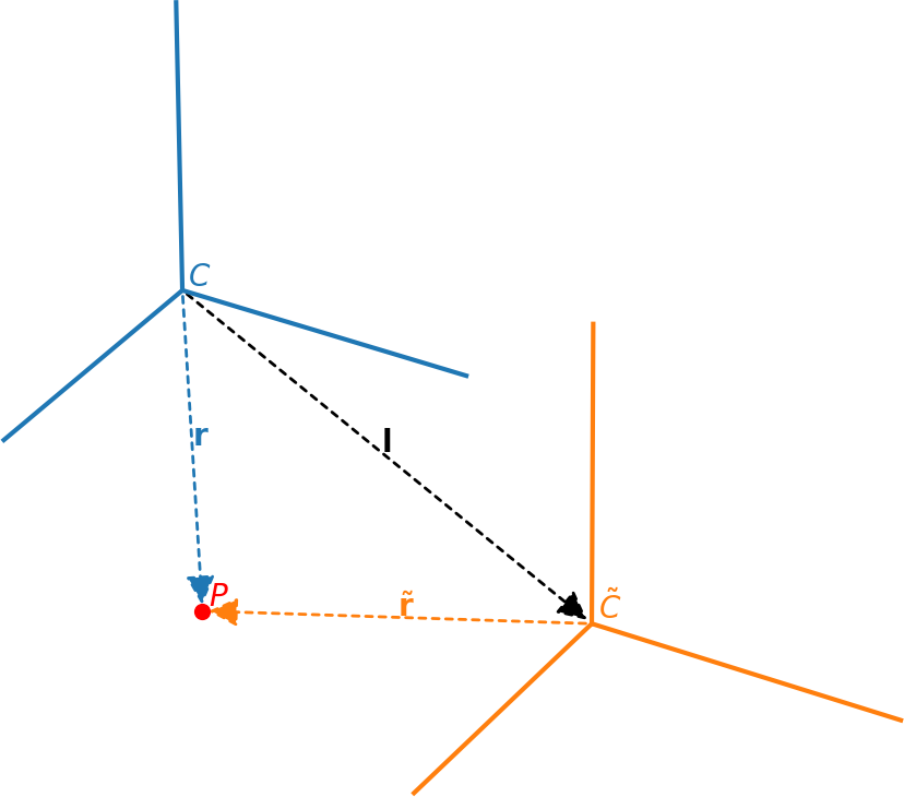
Fig. 5 Inertial frame \(C\) and non-inertial frame \(\tilde{C}\). We consider a fluid element \(P\), whose distance in the two frames is related by \({\bf r} = \tilde{\bf{r}} + {\bf l}\)

Consider an inertial reference frame \(C\) and a non-inertial reference frame \(\widetilde{C}\) whose origins are separated by the vector \(\boldsymbol{l}\) (see the figure above). The non-inertial frame is rotating about the axis \(\ob\) with a constant angular velocity \(\omega\); furthermore, we assume the direction of the rotational axis is fixed. Consider a fluid element at the point \(P\) whose location is given by \(\rb\) in \(C\) and by \(\rbt\) in \(\widetilde{C}\):

\[\rb = \rbt + \boldsymbol{l},\]

or in component notation

(12)\[r_i\boldsymbol{e_i} = \widetilde{r_i}\widetilde{\boldsymbol{e_i}} + l_i\boldsymbol{e_i},\]

where \(\boldsymbol{e_i}\) and \(\widetilde{\boldsymbol{e_i}}\) are the \(i\)th unit vectors in the \(C\) and \(\widetilde{C}\) coordinate systems, respectively. The total time rate of change of (12) is given by

(13)\[\frac{Dr_i}{Dt}\boldsymbol{e_i} = \frac{D\widetilde{r_i}}{Dt}\widetilde{\boldsymbol{e_i}} + \widetilde{r_i}\frac{D\widetilde{\boldsymbol{e_i}}}{Dt} + \frac{Dl_i}{Dt}\boldsymbol{e_i},\]

where we have used the fact that the unit vectors of the inertial frame \(C\) are not moving (or at least can be considered stationary, and the change in \(\boldsymbol{l}\) gives the relative motion of the two coordinate systems). By definition, a unit vector can not change its length, and therefore the only change of \(\widetilde{\boldsymbol{e_i}}\) with time can come from changing direction. This change is carried out by a rotation about the \(\ob\) axis, and the tip of the unit vector moves circumferentially, that is

(14)\[\frac{D\widetilde{\boldsymbol{e_i}}}{Dt} = \ob\times\widetilde{\boldsymbol{e_i}}.\]

Plugging (14) into (13) and switching back to vector notation, we have

(15)\[\frac{D\rb}{Dt} = \frac{D\rbt}{Dt} + \ob\times\rbt + \frac{D\boldsymbol{l}}{Dt}.\]

The left hand side of (15) is interpreted as the velocity of the fluid element as seen in the inertial frame; the first term on the right hand side is the velocity of the fluid element as seen by a stationary observer in the rotating frame \(\widetilde{C}\). The second and third terms on the right hand side of (15) describe the additional velocity due to rotation and translation of the frame \(\widetilde{C}\) as seen in \(C\). In other words,

(16)\[\vb = \vbt + \ob\times\rbt + \boldsymbol{v_l},\]

where we use \(\boldsymbol{v_l}\) to represent the translational velocity.

Similarly, by taking a second time derivative of (16) we have

(17)\[\frac{D\vb}{Dt} = \frac{D\vbt}{Dt} + 2\ob\times\vbt + \ob\times\left[\ob\times\rbt\right] + \frac{D\boldsymbol{v_l}}{Dt}.\]

Henceforth we will assume the two coordinate systems are not translating relative to one another, \(\boldsymbol{v_l} = 0\). It is also worth mentioning that derivatives with respect to spatial coordinates do not involve additional terms due to rotation, i.e. \(\nablab\cdot\vb = \nablab\cdot\vbt\). Because of this, the continuity equation remains unchanged in the rotating frame:

(18)\[\frac{\partial \rho}{\partial t} = -\nablab\cdot\left(\rho\vbt\right),\]

or

(19)\[\frac{D\rho}{Dt} = -\rho\nablab\cdot\vbt.\]

Momentum equation in rotating frame

The usual momentum equation applies in an inertial frame:

(20)\[\frac{D\left(\rho\vb\right)}{Dt} = -\rho\vb\cdot\nablab\vb - \nablab p + \rho\gb.\]

Using the continuity equation, (19), and substituting for the terms in the rotating frame from (17), we have from (20):

\[\begin{split}\begin{align} \rho\left(\frac{D\vbt}{Dt} + 2\ob\times\vbt + \ob\times\left[\ob\times\rbt\right]\right) - \rho\vb\nablab\cdot\vb &= -\rho\vb\cdot\nablab\vb - \nablab p + \rho\gb \nonumber \\ \rho\left(\frac{\partial\vbt}{\partial t} + \vbt\cdot\nablab\vbt\right) &= -\nablab p + \rho\gb - 2\rho\ob\times\vbt - \rho\ob\times\left[\ob\times\rbt\right] \nonumber \\ \frac{\partial\left(\rho\vbt\right)}{\partial t} &= -\nablab\cdot\left(\rho\vbt\vbt\right) - \nablab p + \rho\gb - 2\rho\ob\times\vbt \nonumber \\ &-\ \rho\ob\times\left[\ob\times\rbt\right]\label{eq:mom-rot} \end{align}\end{split}\]

or

(21)\[\frac{D\left(\rho\vbt\right)}{Dt} = -\rho\vbt\cdot\nablab\vbt - \nablab p + \rho\gb - 2\rho\ob\times\vbt - \rho\ob\times\left[\ob\times\rbt\right].\]

Energy equations in rotating frame

From (21), we have the velocity evolution equation in a rotating frame

(22)\[\frac{D\vbt}{Dt} = -\frac{1}{\rho}\nablab p + \gb - 2\ob\times\vbt - \ob\times\left[\ob\times\rbt\right].\]

The kinetic energy equation can be obtained from (22) by multiplying by \(\rho\vbt\):

(23)\[\begin{split}\begin{align} \rho\vbt\cdot\frac{D\vbt}{Dt} &= -\vbt\cdot\nablab p + \rho\vbt\cdot\gb - 2\rho\vbt\cdot\left[\ob\times\vbt\right] - \rho\vbt\cdot\left\{\ob\times\left[\ob\times\rbt\right]\right\} \nonumber \\ \frac{1}{2}\frac{D\left(\rho\vbt\cdot\vbt\right)}{Dt} - \frac{1}{2}\vbt\cdot\vbt\frac{D\rho}{Dt} &= -\vbt\cdot\nablab p + \rho\vbt\cdot\gb - \rho\vbt\cdot\left[\left(\ob\cdot\rbt\right)\ob - \rho\omega^2\rbt\right] \nonumber \\ \frac{1}{2}\frac{D\left(\rho\vbt\cdot\vbt\right)}{Dt} &= -\frac{1}{2}\rho\vbt\cdot\vbt\nablab\cdot\vbt - \vbt\cdot\nablab p + \rho\vbt\cdot\gb - \rho\vbt\cdot\left[\left(\ob\cdot\rbt\right)\ob - \rho\omega^2\rbt\right]. \end{align}\end{split}\]

The internal energy is simply advected, and, from the first law of thermodynamics, can change due to \(pdV\) work:

(24)\[\frac{D\left(\rho e\right)}{Dt} = -\left(\rho e + p\right)\nablab\cdot\vbt.\]

Combining (23) and (24) we can get the evolution of the total specific energy in the rotating frame, \(\rho \widetilde{E} = \rho e + \frac{1}{2}\rho\vbt\cdot\vbt\):

\[\begin{split}\begin{align} \frac{D\left(\rho e\right)}{Dt} + \frac{1}{2}\frac{D\left(\rho\vbt\cdot\vbt\right)}{Dt} &= -\left(\rho e + p + \frac{1}{2}\rho\vbt\cdot\vbt\right)\nablab\cdot\vbt - \vbt\cdot\nablab p \\ & + \rho\vbt\cdot\gb -\rho\vbt\cdot\left[\left(\ob\cdot\rbt\right)\ob - \rho\omega^2\rbt\right]\nonumber \\ \frac{D\left(\rho \widetilde{E}\right)}{Dt} &= -\rho\widetilde{E}\nablab\cdot\vbt - \nablab\cdot\left(p\vbt\right) + \rho\vbt\cdot\gb - \rho\vbt\cdot\left[\left(\ob\cdot\rbt\right)\ob - \rho\omega^2\rbt\right] \label{eq:etot-rot-total} \end{align}\end{split}\]

or

\[\label{eq:etot-rot} \frac{\partial\left(\rho\widetilde{E}\right)}{\partial t} = -\nablab\cdot\left(\rho\widetilde{E}\vbt + p\vbt\right) + \rho\vbt\cdot\gb - \rho\vbt\cdot\left[\left(\ob\cdot\rbt\right)\ob - \rho\omega^2\rbt\right].\]

Switching to the rotating reference frame

If we choose to be a stationary observer in the rotating reference frame, we can drop all of the tildes, which indicated terms in the non-inertial frame \(\widetilde{C}\). Doing so, and making sure we account for the offset, \(\boldsymbol{l}\), between the two coordinate systems, we obtain the following equations for hydrodynamics in a rotating frame of reference:

\[\begin{split}\begin{align} \frac{\partial\rho}{\partial t} &= -\nablab\cdot\left(\rho\vb\right) \label{eq:cont-rot-switch} \\ \frac{\partial \left(\rho\vb\right)}{\partial t} &= -\nablab\cdot\left(\rho\vb\vb\right) - \nablab p + \rho\gb - 2\rho\ob\times\vb - \rho\left(\ob\cdot\rb\right)\ob + \rho\omega^2\rb \label{eq:mom-rot-switch} \\ \frac{\partial\left(\rho E\right)}{\partial t} &= -\nablab\cdot\left(\rho E\vb + p\vb\right) + \rho\vb\cdot\gb - \rho\left(\ob\cdot\rb\right)\left(\ob\cdot\vb\right) + \rho\omega^2\left(\vb\cdot\rb\right). \label{eq:etot-rot-switch} \end{align}\end{split}\]

Adding the forcing to the hydrodynamics

There are several ways to incorporate the effect of the rotation forcing on the hydrodynamical evolution. We control this through the use of the runtime parameter castro.rot_source_type. This is an integer with values currently ranging from 1 through 4, and these values are all analogous to the way that gravity is used to update the momentum and energy. For the most part, the differences are in how the energy update is done:

• castro.rot_source_type = 1 : we use a standard predictor-corrector formalism for updating the momentum and energy. Specifically, our first update is equal to \(\Delta t \times \mathbf{S}^n\) , where \(\mathbf{S}^n\) is the value of the source terms at the old-time (which is usually called time-level \(n\)). At the end of the timestep, we do a corrector step where we subtract off \(\Delta t / 2 \times \mathbf{S}^n\) and add on \(\Delta t / 2 \times \mathbf{S}^{n+1}\), so that at the end of the timestep the source term is properly time centered.

• castro.rot_source_type = 2 : we do something very similar to 1. The major difference is that when evaluating the energy source term at the new time (which is equal to \(\mathbf{u} \cdot \mathbf{S}^{n+1}_{\rho \mathbf{u}}\), where the latter is the momentum source term evaluated at the new time), we first update the momentum, rather than using the value of \(\mathbf{u}\) before entering the rotation source terms. This permits a tighter coupling between the momentum and energy update and we have seen that it usually results in a more accurate evolution.

• castro.rot_source_type = 3 : we do the same momentum update as the previous two, but for the energy update, we put all of the work into updating the kinetic energy alone. In particular, we explicitly ensure that \((rho e)\) maintains the same, and update \((rho K)\) with the work due to rotation, adding the new kinetic energy to the old internal energy to determine the final total gas energy. The physical motivation is that work should be done on the velocity, and should not directly update the temperature – only indirectly through things like shocks.

• castro.rot_source_type = 4the energy update is done in a

  “conservative” fashion. The previous methods all evaluate the value of the source term at the cell center, but this method evaluates the change in energy at cell edges, using the hydrodynamical mass fluxes, permitting total energy to be conserved (excluding possible losses at open domain boundaries). Additionally, the velocity update is slightly different—for the corrector step, we note that there is an implicit coupling between the velocity components, and we directly solve this coupled equation, which results in a slightly better coupling and a more accurate evolution.

The other major option is castro.implicit_rotation_update. This does the update of the Coriolis term in the momentum equation implicitly (e.g., the velocity in the Coriolis force for the zone depends on the updated momentum). The energy update is unchanged.

A detailed discussion of these options and some verification tests is presented in [49].