Hydrodynamics

Introduction

The hydrodynamics scheme in Castro implements an unsplit second-order Godunov method. Characteristic tracing is used to time-center the input states to the Riemann solver. The same hydrodynamics routines are used for pure hydro and radiation hydrodynamics.

Some general notes:

• Regardless of the dimensionality, we always carry around all 3 components of velocity/momentum—this allows for rotation sources easily.

• When radiation is enabled (via RADIATION), we discuss the gas and radiation quantities separately. This generally applies to the temperature, pressure, internal energy, various adiabatic indices, and sound speed. When we refer to the “total” value of one of these, it means that both gas and radiation contributions are included. When we refer to the “gas” quantity, this is what the equation of state would return.

  For continuity, we continue to use the “gas” qualifier even if we are not solving the radiation hydrodynamics equations. In this case, it still means that it comes through the equation of state, but note some of our equations of state (like the helmeos) include a radiation pressure contribution when we are running without radiation hydrodynamics enabled. In this case, we still refer to this as the “gas”.

Hydrodynamics Data Structures

Within the routines that implement the hydrodynamics, there are several main data structures that hold the state.

• conserved state: these arrays generally begin with u, e.g., uin, uout. The NUM_STATE components for the state data in the array are accessed using integer keys defined in Table 6.

  Table 6 The integer variables to index the conservative state array

  variable	quantity	note
  URHO	$\rho$
  UMX	$\rho u$
  UMY	$\rho v$
  UMZ	$\rho w$
  UEDEN	$\rho E$
  UEINT	$\rho e$	this is computed from the other quantities using $\rho e=\rho E-\rho |\mathbf{u}{|}^2/2$
  UTEMP	$T$	this is computed from the other quantities using the EOS
  UFA	$\rho A_1$	the first advected quantity
  UFS	$\rho X_1$	the first species
  UFX	$\rho Y_1$	the first auxiliary variable
  USHK	a shock flag	(used for shock detection)
  UMR	radial momentum	(if HYBRID_MOMENTUM is defined)
  UML	angular momentum	(if HYBRID_MOMENTUM is defined)
  UMP	vertical momentum	(if HYBRID_MOMENTUM is defined)

• primitive variable state: these arrays generally simply called q, and has NQ components.

  A related quantity is NQSRC which is the number of primitive variable source terms. NQSRC ≤ NQ.

  Note

  if RADIATION is defined, then only the gas/hydro terms are present in NQSRC.

  Table 7 gives the names of the primitive variable integer keys for accessing these arrays. Note, unless otherwise specified the quantities without a subscript are “gas” only and those with the “tot” subscript are “gas + radiation”.

  Table 7 Primitive State Vector Integer Keys

  variable	quantity	note
  QRHO	$\rho$
  QU	$u$
  QV	$v$
  QW	$w$
  QPRES	$p$
  QREINT	$\rho e$
  QTEMP	$T$
  QFA	$A_1$	the first advected quantity
  QFS	$X_1$	the first species
  QFX	$Y_1$	the first auxiliary variable
  QPTOT	$p_{\mathrm{tot}}$	the total pressure, gas + radiation
  QREITOT	$e_{\mathrm{tot}}$	the total specific internal energy, gas + radiation
  QRAD	$E_r$	the radiation energy (there are ngroups of these)

• auxiliary primitive variables: these arrays are generally called qaux. The main difference between these and the regular primitive variables is that we do not attempt to do any reconstruction on their profiles. There are NQAUX quantities, indexed by the integer keys listed in Table 8. Note, unless otherwise specified the quantities without a subscript are “gas” only and those with the “tot” subscript are “gas + radiation”.

  Table 8 The integer variable keys for accessing the auxiliary primitive state vector, quax.

  variable	quantity	note
  QGAMC	${\gamma }_1$	the first adiabatic exponent, as returned from the EOS
  QC	$c_s$	the sound speed, as returned from the EOS
  QGAMCG	${{\mathrm{\Gamma }}_1}_{\mathrm{tot}}$	includes radiation components (defined only if RADIATION is defined)
  QCG	${c_s}_{\mathrm{tot}}$	total sound speed including radiation (defined only if RADIATION is defined)
  QLAMS	${\lambda }_f$	the ngroups flux limiters (defined only if RADIATION is defined)

• interface variables: these are the time-centered interface states returned by the Riemann solver. They are used to discretize some non-conservative terms in the equations. These arrays are generally called q1, q2, and q3 for the x, y, and z interfaces respectively. There are NGDNV components accessed with the integer keys defined in Table 9 Note, unless otherwise specified the quantities without a subscript are “gas” only and those with the “tot” subscript are “gas + radiation”.

  Table 9 The integer variable keys for accessing the Godunov interface state vectors.

  variable	quantity	note
  GDRHO	$\rho$
  GDU	$u$
  GDV	$v$
  GDW	$w$
  GDPRES	$p$	regardless of whether RADIATION is defined, this is always just the gas pressure
  GDLAMS	${\lambda }_f$	the starting index for the flux limiter—there are ngroups components (defined only if RADIATION is defined)
  GDERADS	$E_r$	the starting index for the radiation energy—there are ngroups components (defined only if RADIATION is defined)

Conservation Forms

We begin with the fully compressible equations for the conserved state vector, $\mathbf{U}=(\rho ,\rho \mathbf{u},\rho E,\rho A_k,\rho X_k,\rho Y_k):$

$$\begin{array}{r}\begin{array}{rl}\frac{\partial \rho }{\partial t}& =-\mathrm{\nabla }\cdot (\rho \mathbf{u})+S_{\mathrm{e}\mathrm{x}\mathrm{t},\rho },\\ \frac{\partial (\rho \mathbf{u})}{\partial t}& =-\mathrm{\nabla }\cdot (\rho \mathbf{u}\mathbf{u})-\mathrm{\nabla }p+\rho \mathbf{g}+{\mathbf{S}}_{\mathrm{e}\mathrm{x}\mathrm{t},\rho \mathbf{u}},\\ \frac{\partial (\rho E)}{\partial t}& =-\mathrm{\nabla }\cdot (\rho \mathbf{u}E+p\mathbf{u})+\rho \mathbf{u}\cdot \mathbf{g}-\sum _k\rho q_k{\dot{\omega }}_k+\mathrm{\nabla }\cdot k_{\mathrm{th}}\mathrm{\nabla }T+S_{\mathrm{e}\mathrm{x}\mathrm{t},\rho E},\\ \frac{\partial (\rho A_k)}{\partial t}& =-\mathrm{\nabla }\cdot (\rho \mathbf{u}{A}_k)+S_{\mathrm{e}\mathrm{x}\mathrm{t},\rho A_k},\\ \frac{\partial (\rho X_k)}{\partial t}& =-\mathrm{\nabla }\cdot (\rho \mathbf{u}{X}_k)+\rho {\dot{\omega }}_k+S_{\mathrm{e}\mathrm{x}\mathrm{t},\rho X_k},\\ \frac{\partial (\rho Y_k)}{\partial t}& =-\mathrm{\nabla }\cdot (\rho \mathbf{u}{Y}_k)+S_{\mathrm{e}\mathrm{x}\mathrm{t},\rho Y_k}.\end{array}\end{array}$$

Here $\rho ,\mathbf{u},T,p$, and $k_{\mathrm{th}}$ are the density, velocity, temperature, pressure, and thermal conductivity, respectively, and $E=e+\mathbf{u}\cdot \mathbf{u}/2$ is the total energy with $e$ representing the internal energy. In addition, $X_k$ is the abundance of the $k^{\mathrm{t}\mathrm{h}}$ isotope, with associated production rate, ${\dot{\omega }}_k$, and energy release, $q_k$. Here $\mathbf{g}$ is the gravitational vector, and $S_{\mathrm{e}\mathrm{x}\mathrm{t},\rho },{\mathbf{S}}_{\mathrm{e}\mathrm{x}\mathrm{t}\rho \mathbf{u}}$, etc., are user-specified source terms. $A_k$ is an advected quantity, i.e., a tracer. We also carry around auxiliary variables, $Y_k$, which have a user-defined evolution equation, but by default are treated as advected quantities. These are meant to be defined in the network.

In the code we also carry around $T$ and $\rho e$ in the conservative state vector even though they are derived from the other conserved quantities. The ordering of the elements within $\mathbf{U}$ is defined by integer variables into the array—see Table 6.

Some notes:

• Regardless of the dimensionality of the problem, we always carry all 3 components of the velocity. This allows for, e.g., 2.5-d rotation (advecting the component of velocity out of the plane in axisymmetric coordinates).

  You should always initialize all velocity components to zero, and always construct the kinetic energy with all three velocity components.

• There are NADV advected quantities, which range from UFA: UFA+nadv-1. The advected quantities have no effect at all on the rest of the solution but can be useful as tracer quantities.

• There are NSPEC species (defined in the network directory), which range from UFS: UFS+nspec-1.

• There are NAUX auxiliary variables, from UFX:UFX+naux-1. The auxiliary variables are passed into the equation of state routines along with the species. An example of an auxiliary variable is the electron fraction, $Y_e$, in core collapse simulations. The number and names of the auxiliary variables are defined in the network.

Source Terms

We now compute explicit source terms for each variable in $\mathbf{Q}$ and $\mathbf{U}$. The primitive variable source terms will be used to construct time-centered fluxes. The conserved variable source will be used to advance the solution. We neglect reaction source terms since they are accounted for in Steps 1 and 6. The source terms are:

$$\begin{array}{r}{\mathbf{S}}_{\mathbf{Q}}^n={\left(\begin{array}{c}{S}_{\rho }\\ {\mathbf{S}}_{\mathbf{u}}\\ S_p\\ S_{\rho e}\\ S_{A_k}\\ S_{X_k}\\ S_{Y_k}\end{array}\right)}^n={\left(\begin{array}{c}{S}_{\mathrm{e}\mathrm{x}\mathrm{t},\rho }\\ \mathbf{g}+\frac{1}{\rho }{\mathbf{S}}_{\mathrm{e}\mathrm{x}\mathrm{t},\rho \mathbf{u}}\\ \frac{1}{\rho }\frac{\partial p}{\partial e}{S}_{\mathrm{e}\mathrm{x}\mathrm{t},\rho E}+\frac{\partial p}{\partial \rho }{S}_{\mathrm{e}\mathrm{x}\mathrm{t}\rho }\\ \mathrm{\nabla }\cdot k_{\mathrm{th}}\mathrm{\nabla }T+S_{\mathrm{e}\mathrm{x}\mathrm{t},\rho E}\\ \frac{1}{\rho }{S}_{\mathrm{e}\mathrm{x}\mathrm{t},\rho A_k}\\ \frac{1}{\rho }{S}_{\mathrm{e}\mathrm{x}\mathrm{t},\rho X_k}\\ \frac{1}{\rho }{S}_{\mathrm{e}\mathrm{x}\mathrm{t},\rho Y_k}\end{array}\right)}^n,\end{array}$$

$$\begin{array}{r}{\mathbf{S}}_{\mathbf{U}}^n={\left(\begin{array}{c}{\mathbf{S}}_{\rho \mathbf{u}}\\ S_{\rho E}\\ S_{\rho A_k}\\ S_{\rho X_k}\\ S_{\rho Y_k}\end{array}\right)}^n={\left(\begin{array}{c}\rho \mathbf{g}+{\mathbf{S}}_{\mathrm{e}\mathrm{x}\mathrm{t},\rho \mathbf{u}}\\ \rho \mathbf{u}\cdot \mathbf{g}+\mathrm{\nabla }\cdot k_{\mathrm{th}}\mathrm{\nabla }T+S_{\mathrm{e}\mathrm{x}\mathrm{t},\rho E}\\ S_{\mathrm{e}\mathrm{x}\mathrm{t},\rho A_k}\\ S_{\mathrm{e}\mathrm{x}\mathrm{t},\rho X_k}\\ S_{\mathrm{e}\mathrm{x}\mathrm{t},\rho Y_k}\end{array}\right)}^n.\end{array}$$

Note

To reduce memory usage, we do not include source terms for the advected quantities, species, and auxiliary variables in the conserved state vector by default. If your application needs external source terms for these variables, set USE_SPECIES_SOURCES=TRUE when compiling so that space will be allocated for them.

Primitive Forms

Castro uses the primitive form of the fluid equations, defined in terms of the state $\mathbf{Q}=(\rho ,\mathbf{u},p,\rho e,A_k,X_k,Y_k)$, to construct the interface states that are input to the Riemann problem.

The primitive variable equations for density, velocity, and pressure are:

$$\begin{array}{r}\begin{array}{rl}\frac{\partial \rho }{\partial t}& =-\mathbf{u}\cdot \mathrm{\nabla }\rho -\rho \mathrm{\nabla }\cdot \mathbf{u}+S_{\mathrm{e}\mathrm{x}\mathrm{t},\rho }\\ \frac{\partial \mathbf{u}}{\partial t}& =-\mathbf{u}\cdot \mathrm{\nabla }\mathbf{u}-\frac{1}{\rho }\mathrm{\nabla }p+\mathbf{g}+\frac{1}{\rho }({\mathbf{S}}_{\mathrm{e}\mathrm{x}\mathrm{t},\rho \mathbf{u}}-\mathbf{u}{S}_{\mathrm{e}\mathrm{x}\mathrm{t},\rho })\\ \frac{\partial p}{\partial t}& =-\mathbf{u}\cdot \mathrm{\nabla }p-\rho c^2\mathrm{\nabla }\cdot \mathbf{u}+{\left(\frac{\partial p}{\partial \rho }\right)}_{e,X}{S}_{\mathrm{e}\mathrm{x}\mathrm{t},\rho }\\ & +\frac{1}{\rho }\sum _k{\left(\frac{\partial p}{\partial X_k}\right)}_{\rho ,e,X_j,j\ne k}(\rho {\dot{\omega }}_k+S_{\mathrm{e}\mathrm{x}\mathrm{t},\rho X_k}-X_k{S}_{\mathrm{e}\mathrm{x}\mathrm{t},\rho })\\ & +\frac{1}{\rho }{\left(\frac{\partial p}{\partial e}\right)}_{\rho ,X}[-e{S}_{\mathrm{e}\mathrm{x}\mathrm{t},\rho }-\sum _k\rho q_k{\dot{\omega }}_k+\mathrm{\nabla }\cdot k_{\mathrm{th}}\mathrm{\nabla }T\\ & +S_{\mathrm{e}\mathrm{x}\mathrm{t},\rho E}-\mathbf{u}\cdot ({\mathbf{S}}_{\mathrm{e}\mathrm{x}\mathrm{t},\rho \mathbf{u}}-\frac{\mathbf{u}}{2}{S}_{\mathrm{e}\mathrm{x}\mathrm{t},\rho })]\end{array}\end{array}$$

The advected quantities appear as:

$$\begin{array}{r}\begin{array}{rl}\frac{\partial A_k}{\partial t}& =-\mathbf{u}\cdot \mathrm{\nabla }{A}_k+\frac{1}{\rho }(S_{\mathrm{e}\mathrm{x}\mathrm{t},\rho A_k}-A_k{S}_{\mathrm{e}\mathrm{x}\mathrm{t},\rho }),\\ \frac{\partial X_k}{\partial t}& =-\mathbf{u}\cdot \mathrm{\nabla }{X}_k+{\dot{\omega }}_k+\frac{1}{\rho }(S_{\mathrm{e}\mathrm{x}\mathrm{t},\rho X_k}-X_k{S}_{\mathrm{e}\mathrm{x}\mathrm{t},\rho }),\\ \frac{\partial Y_k}{\partial t}& =-\mathbf{u}\cdot \mathrm{\nabla }{Y}_k+\frac{1}{\rho }(S_{\mathrm{e}\mathrm{x}\mathrm{t},\rho Y_k}-Y_k{S}_{\mathrm{e}\mathrm{x}\mathrm{t},\rho }).\end{array}\end{array}$$

All of the primitive variables are derived from the conservative state vector, as described in Section 6.1. When accessing the primitive variable state vector, the integer variable keys for the different quantities are listed in Table 7.

Internal energy and temperature

We augment the above system with an internal energy equation:

$$\begin{array}{r}\begin{array}{rl}\frac{\partial (\rho e)}{\partial t}& =-\mathbf{u}\cdot \mathrm{\nabla }(\rho e)-(\rho e+p)\mathrm{\nabla }\cdot \mathbf{u}-\sum _k\rho q_k{\dot{\omega }}_k+\mathrm{\nabla }\cdot k_{\mathrm{th}}\mathrm{\nabla }T+S_{\mathrm{e}\mathrm{x}\mathrm{t},\rho E}\\ & -\mathbf{u}\cdot ({\mathbf{S}}_{\mathrm{e}\mathrm{x}\mathrm{t},\rho \mathbf{u}}-\frac{1}{2}{S}_{\mathrm{e}\mathrm{x}\mathrm{t},\rho }\mathbf{u}),\end{array}\end{array}$$

This has two benefits. First, for a general equation of state, carrying around an additional thermodynamic quantity allows us to avoid equation of state calls (in particular, in the Riemann solver, see e.g. [28]). Second, it is sometimes the case that the internal energy calculated as

$$e_T\equiv E-\frac{1}{2}{\mathbf{v}}^2$$

is unreliable. This has two usual causes: one, for high Mach number flows, the kinetic energy can dominate the total gas energy, making the subtraction numerically unreliable; two, if you use gravity or other source terms, these can indirectly alter the value of the internal energy if obtained from the total energy.

To provide a more reasonable internal energy for defining the thermodynamic state, we have implemented the dual energy formalism from ENZO [24], [23], where we switch between $(\rho e)$ and $(\rho e_T)$ depending on the local state of the fluid. To do so, we define parameters ${\eta }_1$, ${\eta }_2$, and ${\eta }_3$, corresponding to the code parameters castro.dual_energy_eta1, castro.dual_energy_eta2, and castro.dual_energy_eta3. We then consider the ratio $e_T/E$, the ratio of the internal energy (derived from the total energy) to the total energy. These parameters are used as follows:

• ${\eta }_1$: If $e_T>{\eta }_{1}E$, then we use $e_T$ for the purpose of calculating the pressure in the hydrodynamics update. Otherwise, we use the $e$ from the internal energy equation in our EOS call to get the pressure.

• ${\eta }_2$: At the end of each hydro advance, we examine whether $e_T>{\eta }_{2}E$. If so, we reset $e$ to be equal to $e_T$, discarding the results of the internal energy equation. Otherwise, we keep $e$ as it is.

• ${\eta }_3$: Similar to ${\eta }_1$, if $e_T>{\eta }_{3}E$, we use $e_T$ for the purposes of our nuclear reactions, otherwise, we use $e$.

Note that our version of the internal energy equation does not require an artificial viscosity, as used in some other hydrodynamics codes. The update for $(\rho e)$ uses information from the Riemann solve to calculate the fluxes, which contains the information intrinsic to the shock-capturing part of the scheme.

In the code we also carry around $T$ in the primitive state vector.

Primitive Variable System

The full primitive variable form (without the advected or auxiliary quantities) is

$$\frac{\partial \mathbf{Q}}{\partial t}+\sum _d{\mathbf{A}}_d\frac{\partial \mathbf{Q}}{\partial x_d}={\mathbf{S}}_{\mathbf{Q}}.$$

For example, in 2D:

$$\begin{array}{r}{\left(\begin{array}{c}\rho \\ u\\ v\\ p\\ \rho e\\ X_k\end{array}\right)}_t+\left(\begin{array}{cccccc}u& \rho & 0& 0& 0& 0\\ 0& u& 0& \frac{1}{\rho }& 0& 0\\ 0& 0& u& 0& 0& 0\\ 0& \rho c^2& 0& u& 0& 0\\ 0& \rho e+p& 0& 0& u& 0\\ 0& 0& 0& 0& 0& u\end{array}\right){\left(\begin{array}{c}\rho \\ u\\ v\\ p\\ \rho e\\ X_k\end{array}\right)}_x+\left(\begin{array}{cccccc}v& 0& \rho & 0& 0& 0\\ 0& v& 0& 0& 0& 0\\ 0& 0& v& \frac{1}{\rho }& 0& 0\\ 0& 0& \rho c^2& v& 0& 0\\ 0& 0& \rho e+p& 0& v& 0\\ 0& 0& 0& 0& 0& v\end{array}\right){\left(\begin{array}{c}\rho \\ u\\ v\\ p\\ \rho e\\ X_k\end{array}\right)}_y={\mathbf{S}}_{\mathbf{Q}}\end{array}$$

The eigenvalues are:

$$\mathbf{\Lambda }({\mathbf{A}}_x)=\{u-c,u,u,u,u,u+c\},\mathbf{\Lambda }({\mathbf{A}}_y)=\{v-c,v,v,v,v,v+c\}.$$

The right column eigenvectors are:

$$\begin{array}{r}\mathbf{R}({\mathbf{A}}_x)=\left(\begin{array}{cccccc}1& 1& 0& 0& 0& 1\\ -\frac{c}{\rho }& 0& 0& 0& 0& \frac{c}{\rho }\\ 0& 0& 1& 0& 0& 0\\ c^2& 0& 0& 0& 0& c^2\\ h& 0& 0& 1& 0& h\\ 0& 0& 0& 0& 1& 0\end{array}\right),\mathbf{R}({\mathbf{A}}_y)=\left(\begin{array}{cccccc}1& 1& 0& 0& 0& 1\\ 0& 0& 1& 0& 0& 0\\ -\frac{c}{\rho }& 0& 0& 0& 0& \frac{c}{\rho }\\ c^2& 0& 0& 0& 0& c^2\\ h& 0& 0& 1& 0& h\\ 0& 0& 0& 0& 1& 0\end{array}\right).\end{array}$$

The left row eigenvectors, normalized so that ${\mathbf{R}}_d\cdot {\mathbf{L}}_d=\mathbf{I}$ are:

$$\begin{array}{r}{\mathbf{L}}_x=\left(\begin{array}{cccccc}0& -\frac{\rho }{2c}& 0& \frac{1}{2c^2}& 0& 0\\ 1& 0& 0& -\frac{1}{c^2}& 0& 0\\ 0& 0& 1& 0& 0& 0\\ 0& 0& 0& -\frac{h}{c^2}& 1& 0\\ 0& 0& 0& 0& 0& 1\\ 0& \frac{\rho }{2c}& 0& \frac{1}{2c^2}& 0& 0\end{array}\right),{\mathbf{L}}_y=\left(\begin{array}{cccccc}0& 0& -\frac{\rho }{2c}& \frac{1}{2c^2}& 0& 0\\ 1& 0& 0& -\frac{1}{c^2}& 0& 0\\ 0& 1& 0& 0& 0& 0\\ 0& 0& 0& -\frac{h}{c^2}& 1& 0\\ 0& 0& 0& 0& 0& 1\\ 0& 0& \frac{\rho }{2c}& \frac{1}{2c^2}& 0& 0\end{array}\right).\end{array}$$

Hydrodynamics Update

There are four major steps in the hydrodynamics update:

1. Converting to primitive variables

2. Construction the edge states

3. Solving the Riemann problem

4. Doing the conservative update

Each of these steps has a variety of runtime parameters that affect their behavior. Additionally, there are some general runtime parameters for hydrodynamics:

• castro.do_hydro: time-advance the fluid dynamical equations (0 or 1; must be set)

• castro.add_ext_src: include additional user-specified source term (0 or 1; default 0)

• castro.do_sponge: call the sponge routine after the solution update (0 or 1; default: 0)

  See Sponge for more details on the sponge.

Several floors are imposed on the thermodynamic quantities to prevet unphysical behavior:

• castro.small_dens: (Real; default: -1.e20)

• castro.small_temp: (Real; default: -1.e20)

• castro.small_pres: (Real; default: -1.e20)

Compute Primitive Variables

We compute the primitive variables from the conserved variables.

• $\rho ,\rho e$: directly copy these from the conserved state vector

• $\mathbf{u},A_k,X_k,Y_k$: copy these from the conserved state vector, dividing by $\rho$

• $p,T$: use the EOS.

  First, we use the EOS to ensure $e$ is no smaller than $e(\rho ,T_{\mathrm{s}\mathrm{m}\mathrm{a}\mathrm{l}\mathrm{l}},X_k)$. Then we use the EOS to compute $p,T=p,T(\rho ,e,X_k)$.

We also compute the flattening coefficient, $\chi \in [0,1]$, used in the edge state prediction to further limit slopes near strong shocks. We use the same flattening procedure described in the the the original PPM paper [30] and the Flash paper [38]. A flattening coefficient of 1 indicates that no additional limiting takes place; a flattening coefficient of 0 means we effectively drop order to a first-order Godunov scheme (this convention is opposite of that used in the Flash paper). For each cell, we compute the flattening coefficient for each spatial direction, and choose the minimum value over all directions. As an example, to compute the flattening for the x-direction, here are the steps:

1. Define $\zeta$

   $${\zeta }_i=\frac{p_{i+1}-p_{i-1}}{max(p_{\mathrm{s}\mathrm{m}\mathrm{a}\mathrm{l}\mathrm{l}},|p_{i+2}-p_{i-2}|)}.$$

2. Define $\tilde{\chi }$

   $${\tilde{\chi }}_i=min\{1,max[0,a({\zeta }_i-b)]\},$$

   where $a=10$ and $b=0.75$ are tunable parameters. We are essentially setting ${\tilde{\chi }}_i=a({\zeta }_i-b)$, and then constraining ${\tilde{\chi }}_i$ to lie in the range $[0,1]$. Then, if either $u_{i+1}-u_{i-1}<0$ or

   $$\frac{p_{i+1}-p_{i-1}}{min(p_{i+1},p_{i-1})}\le c,$$

   where $c=1/3$ is a tunable parameter, then set ${\tilde{\chi }}_i=0$.

3. Define $\chi$

   $$\begin{array}{r}{\chi }_i=\{\begin{array}{ll}1-max({\tilde{\chi }}_i,{\tilde{\chi }}_{i-1})& p_{i+1}-p_{i-1}>0\\ 1-max({\tilde{\chi }}_i,{\tilde{\chi }}_{i+1})& \text{otherwise}\end{array}.\end{array}$$

The following runtime parameters affect the behavior here:

• castro.use_flattening turns on/off the flattening of parabola near shocks (0 or 1; default 1)

Edge State Prediction

We wish to compute a left and right state of primitive variables at each edge to be used as inputs to the Riemann problem. There are several reconstruction techniques, a piecewise linear method that follows the description in [27], the classic PPM limiters [30], and the new PPM limiters introduced in [29]. The choice of limiters is determined by castro.ppm_type.

For the new PPM limiters, we have further modified the method of [29] to eliminate sensitivity due to roundoff error (modifications via personal communication with Colella).

We also use characteristic tracing with corner coupling in 3D, as described in Miller & Colella (2002) [54]. We give full details of the new PPM algorithm, as it has not appeared before in the literature, and summarize the developments from Miller & Colella.

The PPM algorithm is used to compute time-centered edge states by extrapolating the base-time data in space and time. The edge states are dual-valued, i.e., at each face, there is a left state and a right state estimate. The spatial extrapolation is one-dimensional, i.e., transverse derivatives are ignored. We also use a flattening procedure to further limit the edge state values. The Miller & Colella algorithm, which we describe later, incorporates the transverse terms, and also describes the modifications required for equations with additional characteristics besides the fluid velocity. There are four steps to compute these dual-valued edge states (here, we use $s$ to denote an arbitrary scalar from $\mathbf{Q}$, and we write the equations in 1D, for simplicity):

• Step 1: Compute $s_{i,+}$ and $s_{i,-}$, which are spatial interpolations of $s$ to the hi and lo side of the face with special limiters, respectively. Begin by interpolating $s$ to edges using a 4th-order interpolation in space:

  $$s_{i+\frac{1}{2}}=\frac{7}{12}(s_{i+1}+s_i)-\frac{1}{12}(s_{i+2}+s_{i-1}).$$

  Then, if $(s_{i+\frac{1}{2}}-s_i)(s_{i+1}-s_{i+\frac{1}{2}})<0$, we limit $s_{i+\frac{1}{2}}$ a nonlinear combination of approximations to the second derivative. The steps are as follows:

  1. Define:

     $$\begin{array}{r}\begin{array}{rl}(D^{2}s{)}_{i+\frac{1}{2}}& =3(s_i-2s_{i+\frac{1}{2}}+s_{i+1})\\ (D^{2}s{)}_{i+\frac{1}{2},L}& =s_{i-1}-2s_i+s_{i+1}\\ (D^{2}s{)}_{i+\frac{1}{2},R}& =s_i-2s_{i+1}+s_{i+2}\end{array}\end{array}$$

  2. Define

     $$s=\text{sign}[(D^{2}s{)}_{i+\frac{1}{2}}],$$
     $$(D^{2}s{)}_{i+\frac{1}{2},\text{lim}}=smax\{min[Cs|(D^{2}s{)}_{i+\frac{1}{2},L}|,Cs|(D^{2}s{)}_{i+\frac{1}{2},R}|,s|(D^{2}s{)}_{i+\frac{1}{2}}|],0\},$$

     where $C=1.25$ as used in Colella and Sekora 2009. The limited value of $s_{i+\frac{1}{2}}$ is

     $$s_{i+\frac{1}{2}}=\frac{1}{2}(s_i+s_{i+1})-\frac{1}{6}(D^{2}s{)}_{i+\frac{1}{2},\text{lim}}.$$

  Now we implement an updated implementation of the Colella & Sekora algorithm which eliminates sensitivity to roundoff. First we need to detect whether a particular cell corresponds to an “extremum”. There are two tests.

  • For the first test, define

    $${\alpha }_{i,\pm }=s_{i\pm \frac{1}{2}}-s_i.$$

    If ${\alpha }_{i,+}{\alpha }_{i,-}\ge 0$, then we are at an extremum.

  • We only apply the second test if either $|{\alpha }_{i,\pm }|>2|{\alpha }_{i,\mp }|$. If so, we define:

    $$\begin{array}{r}\begin{array}{rl}(Ds{)}_{i,\mathrm{f}\mathrm{a}\mathrm{c}\mathrm{e},-}& =s_{i-1/2}-s_{i-3/2}\\ (Ds{)}_{i,\mathrm{f}\mathrm{a}\mathrm{c}\mathrm{e},+}& =s_{i+3/2}-s_{i-1/2}\end{array}\end{array}$$
    $$(Ds{)}_{i,\mathrm{f}\mathrm{a}\mathrm{c}\mathrm{e},\mathrm{m}\mathrm{i}\mathrm{n}}=min[|(Ds{)}_{i,\mathrm{f}\mathrm{a}\mathrm{c}\mathrm{e},-}|,|(Ds{)}_{i,\mathrm{f}\mathrm{a}\mathrm{c}\mathrm{e},+}|].$$
    $$\begin{array}{r}\begin{array}{rl}(Ds{)}_{i,\mathrm{c}\mathrm{c},-}& =s_i-s_{i-1}\\ (Ds{)}_{i,\mathrm{c}\mathrm{c},+}& =s_{i+1}-s_i\end{array}\end{array}$$
    $$(Ds{)}_{i,\mathrm{c}\mathrm{c},\mathrm{m}\mathrm{i}\mathrm{n}}=min[|(Ds{)}_{i,\mathrm{c}\mathrm{c},-}|,|(Ds{)}_{i,\mathrm{c}\mathrm{c},+}|].$$

    If $(Ds{)}_{i,\mathrm{f}\mathrm{a}\mathrm{c}\mathrm{e},\mathrm{m}\mathrm{i}\mathrm{n}}\ge (Ds{)}_{i,\mathrm{c}\mathrm{c},\mathrm{m}\mathrm{i}\mathrm{n}}$, set $(Ds{)}_{i,\pm }=(Ds{)}_{i,\mathrm{f}\mathrm{a}\mathrm{c}\mathrm{e},\pm }$. Otherwise, set $(Ds{)}_{i,\pm }=(Ds{)}_{i,\mathrm{c}\mathrm{c},\pm }$. Finally, we are at an extreumum if $(Ds{)}_{i,+}(Ds{)}_{i,-}\le 0$.

  Thus concludes the extremum tests. The remaining limiters depend on whether we are at an extremum.

  • If we are at an extremum, we modify ${\alpha }_{i,\pm }$. First, we define

    $$\begin{array}{r}\begin{array}{rl}(D^{2}s{)}_i& =6({\alpha }_{i,+}+{\alpha }_{i,-})\\ (D^{2}s{)}_{i,L}& =s_{i-2}-2s_{i-1}+s_i\\ (D^{2}s{)}_{i,R}& =s_i-2s_{i+1}+s_{i+2}\\ (D^{2}s{)}_{i,C}& =s_{i-1}-2s_i+s_{i+1}\end{array}\end{array}$$

    Then, define

    $$s=\text{sign}[(D^{2}s{)}_i],$$
    $$(D^{2}s{)}_{i,\text{lim}}=max\{min[s(D^{2}s{)}_i,Cs|(D^{2}s{)}_{i,L}|,Cs|(D^{2}s{)}_{i,R}|,Cs|(D^{2}s{)}_{i,C}|],0\}.$$

    Then,

    $${\alpha }_{i,\pm }=\frac{{\alpha }_{i,\pm }(D^{2}s{)}_{i,\text{lim}}}{max[(D^{2}s{)}_i,1\times {10}^{-10}]}$$

  • If we are not at an extremum and $|{\alpha }_{i,\pm }|>2|{\alpha }_{i,\mp }|$, then define

    $$s=\text{sign}({\alpha }_{i,\mp })$$
    $$\delta {\mathcal{I}}_{\text{ext}}=\frac{-{\alpha }_{i,\pm }^2}{4({\alpha }_{j,+}+{\alpha }_{j,-})},$$
    $$\delta s=s_{i\mp 1}-s_i,$$

    If $s\delta {\mathcal{I}}_{\text{ext}}\ge s\delta s$, then we perform the following test. If $s\delta s-{\alpha }_{i,\mp }\ge 1\times {10}^{-10}$, then

    $${\alpha }_{i,\pm }=-2\delta s-2s{[(\delta s{)}^2-\delta s{\alpha }_{i,\mp }]}^{\frac{1}{2}}$$

    otherwise,

    $${\alpha }_{i,\pm }=-2{\alpha }_{i,\mp }$$

  Finally, $s_{i,\pm }=s_i+{\alpha }_{i,\pm }$.

• Step 2: Construct a quadratic profile using $s_{i,-},s_i$, and $s_{i,+}$.

  (3)$$s_i^I(x)=s_{i,-}+\xi [s_{i,+}-s_{i,-}+s_{6,i}(1-\xi )],$$
  $$s_6=6s_i-3(s_{i,-}+s_{i,+}),$$
  $$\xi =\frac{x-ih}{h},0\le \xi \le 1.$$
• Step 3: Integrate quadratic profiles. We are essentially computing the average value swept out by the quadratic profile across the face assuming the profile is moving at a speed ${\lambda }_k$.

  Define the following integrals, where ${\sigma }_k=|{\lambda }_k|\mathrm{\Delta }t/h$:

  $$\begin{array}{r}\begin{array}{rl}{\mathcal{I}}_{+}^{(k)}(s_i)& =\frac{1}{{\sigma }_{k}h}{\int }_{(i+\frac{1}{2})h-{\sigma }_{k}h}^{(i+\frac{1}{2})h}{s}_i^I(x)dx\\ {\mathcal{I}}_{-}^{(k)}(s_i)& =\frac{1}{{\sigma }_{k}h}{\int }_{(i-\frac{1}{2})h}^{(i-\frac{1}{2})h+{\sigma }_{k}h}{s}_i^I(x)dx\end{array}\end{array}$$

  Plugging in (3) gives:

  $$\begin{array}{r}\begin{array}{rl}{\mathcal{I}}_{+}^{(k)}(s_i)& =s_{i,+}-\frac{{\sigma }_k}{2}[s_{i,+}-s_{i,-}-(1-\frac{2}{3}{\sigma }_k)s_{6,i}],\\ {\mathcal{I}}_{-}^{(k)}(s_i)& =s_{i,-}+\frac{{\sigma }_k}{2}[s_{i,+}-s_{i,-}+(1-\frac{2}{3}{\sigma }_k)s_{6,i}].\end{array}\end{array}$$

• Step 4: Obtain 1D edge states by performing a 1D extrapolation to get left and right edge states. Note that we include an explicit source term contribution.

  $$\begin{array}{r}\begin{array}{rl}{s}_{L,i+\frac{1}{2}}& =s_i-{\chi }_i\sum _{k:{\lambda }_k\ge 0}{\mathbf{l}}_k\cdot [s_i-{\mathcal{I}}_{+}^{(k)}(s_i)]{\mathbf{r}}_k+\frac{\mathrm{\Delta }t}{2}{S}_i^n,\\ s_{R,i-\frac{1}{2}}& =s_i-{\chi }_i\sum _{k:{\lambda }_k<0}{\mathbf{l}}_k\cdot [s_i-{\mathcal{I}}_{-}^{(k)}(s_i)]{\mathbf{r}}_k+\frac{\mathrm{\Delta }t}{2}{S}_i^n.\end{array}\end{array}$$

  Here, ${\mathbf{r}}_k$ is the $k^{\mathrm{t}\mathrm{h}}$ right column eigenvector of $\mathbf{R}({\mathbf{A}}_d)$ and ${\mathbf{l}}_k$ is the $k^{\mathrm{t}\mathrm{h}}$ left row eigenvector lf $\mathbf{L}({\mathbf{A}}_d)$. The flattening coefficient is ${\chi }_i$.

In order to add the transverse terms in an spatial operator unsplit framework, the details follow exactly as given in Section 4.2.1 in Miller & Colella, except for the details of the Riemann solver, which are given below.

For the reconstruction of the interface states, the following apply:

• castro.ppm_type : use piecewise linear vs PPM algorithm (0 or 1; default: 1). A value of 1 is the standard piecewise parabolic reconstruction.

• castro.ppm_temp_fix does various attempts to use the temperature in the reconstruction of the interface states. See Temperature Fixes for an explanation of the allowed options.

The interface states are corrected with information from the transverse directions to make this a second-order update. These transverse directions involve separate Riemann solves. Sometimes, the update to the interface state from the transverse directions can make the state ill-posed. There are several parameters that help fix this:

• castro.transverse_use_eos : If this is 1, then we call the equation of state on the interface, using $\rho$, $e$, and $X_k$, to get the interface pressure. This should result in a thermodynamically consistent interface state.

• castro.transverse_reset_density : If the transverse corrections result in a negative density on the interface, then we reset all of the interface states to their values before the transverse corrections.

• castro.transverse_reset_rhoe : The transverse updates operate on the conserved state. Usually, we construct the interface $(\rho e)$ in the transverse update from total energy and the kinetic energy, however, if the interface $(rhoe)$ is negative, and transverse_reset_rhoe = 1, then we explicitly discretize an equation for the evolution of $(\rho e)$, including its transverse update.

Riemann Problem

Castro has three main options for the Riemann solver—the Colella & Glaz solver [28] (the same solver used by Flash), a simpler solver described in an unpublished manuscript by Colella, Glaz, & Ferguson, and an HLLC solver. The first two are both two-shock approximate solvers, but differ in how they approximate the thermodynamics in the “star” region.

Note

These Riemann solvers are for Newtonian hydrodynamics, however, we enforce that the interface velocity cannot exceed the speed of light in both the Colella & Glaz and Colella, Glaz, & Ferguson solvers. This excessive speed usually is a sign of low density regions and density resets or the flux limiter kicking in. This behavior can be changed with the castro.riemann_speed_limit parameter.

Inputs from the edge state prediction are ${\rho }_{L/R},u_{L/R},v_{L/R},p_{L/R}$, and $(\rho e{)}_{L/R}$ ($v$ represents all of the transverse velocity components). We also compute $\mathrm{\Gamma }\equiv d\log p/d\log \rho {|}_s$ at cell centers and copy these to edges directly to get the left and right states, ${\mathrm{\Gamma }}_{L/R}$. We also define $c_{\mathrm{a}\mathrm{v}\mathrm{g}}$ as a face-centered value that is the average of the neighboring cell-centered values of $c$. We have also computed ${\rho }_{\mathrm{s}\mathrm{m}\mathrm{a}\mathrm{l}\mathrm{l}},p_{\mathrm{s}\mathrm{m}\mathrm{a}\mathrm{l}\mathrm{l}}$, and $c_{\mathrm{s}\mathrm{m}\mathrm{a}\mathrm{l}\mathrm{l}}$ using cell-centered data.

Here are the steps. First, define $(\rho c{)}_{\mathrm{s}\mathrm{m}\mathrm{a}\mathrm{l}\mathrm{l}}={\rho }_{\mathrm{s}\mathrm{m}\mathrm{a}\mathrm{l}\mathrm{l}}{c}_{\mathrm{s}\mathrm{m}\mathrm{a}\mathrm{l}\mathrm{l}}$. Then, define:

$$(\rho c{)}_{L/R}=max[(\rho c{)}_{\mathrm{s}\mathrm{m}\mathrm{a}\mathrm{l}\mathrm{l}},|{\mathrm{\Gamma }}_{L/R},p_{L/R},{\rho }_{L/R}|].$$

Define star states:

$$p^{\ast }=max[p_{\mathrm{s}\mathrm{m}\mathrm{a}\mathrm{l}\mathrm{l}},\frac{[(\rho c{)}_L{p}_R+(\rho c{)}_R{p}_L]+(\rho c{)}_L(\rho c{)}_R(u_L-u_R)}{(\rho c{)}_L+(\rho c{)}_R}],$$

$$u^{\ast }=\frac{[(\rho c{)}_L{u}_L+(\rho c{)}_R{u}_R]+(p_L-p_R)}{(\rho c{)}_L+(\rho c{)}_R}.$$

If $u^{\ast }\ge 0$ then define ${\rho }_0,u_0,p_0,(\rho e{)}_0$ and ${\mathrm{\Gamma }}_0$ to be the left state. Otherwise, define them to be the right state. Then, set

$${\rho }_0=max({\rho }_{\mathrm{s}\mathrm{m}\mathrm{a}\mathrm{l}\mathrm{l}},{\rho }_0),$$

and define

$$c_0=max(c_{\mathrm{s}\mathrm{m}\mathrm{a}\mathrm{l}\mathrm{l}},\sqrt{\frac{{\mathrm{\Gamma }}_0{p}_0}{{\rho }_0}}),$$

$${\rho }^{\ast }={\rho }_0+\frac{p^{\ast }-p_0}{c_0^2},$$

$$(\rho e{)}^{\ast }=(\rho e{)}_0+(p^{\ast }-p_0)\frac{(\rho e{)}_0+p_0}{{\rho }_0{c}_0^2},$$

$$c^{\ast }=max(c_{\mathrm{s}\mathrm{m}\mathrm{a}\mathrm{l}\mathrm{l}},\sqrt{\left|\frac{{\mathrm{\Gamma }}_0{p}^{\ast }}{{\rho }^{\ast }}\right|})$$

Then,

$$\begin{array}{r}\begin{array}{rl}{c}_{\mathrm{o}\mathrm{u}\mathrm{t}}& =c_0-\mathrm{s}\mathrm{i}\mathrm{g}\mathrm{n}(u^{\ast })u_0,\\ c_{\mathrm{i}\mathrm{n}}& =c^{\ast }-\mathrm{s}\mathrm{i}\mathrm{g}\mathrm{n}(u^{\ast })u^{\ast },\\ c_{\mathrm{s}\mathrm{h}\mathrm{o}\mathrm{c}\mathrm{k}}& =\frac{c_{\mathrm{i}\mathrm{n}}+c_{\mathrm{o}\mathrm{u}\mathrm{t}}}{2}.\end{array}\end{array}$$

If $p^{\ast }-p_0\ge 0$, then $c_{\mathrm{i}\mathrm{n}}=c_{\mathrm{o}\mathrm{u}\mathrm{t}}=c_{\mathrm{s}\mathrm{h}\mathrm{o}\mathrm{c}\mathrm{k}}$. Then, if $c_{\mathrm{o}\mathrm{u}\mathrm{t}}=c_{\mathrm{i}\mathrm{n}}$, we define $c_{\mathrm{t}\mathrm{e}\mathrm{m}\mathrm{p}}=ϵc_{\mathrm{a}\mathrm{v}\mathrm{g}}$. Otherwise, $c_{\mathrm{t}\mathrm{e}\mathrm{m}\mathrm{p}}=c_{\mathrm{o}\mathrm{u}\mathrm{t}}-c_{\mathrm{i}\mathrm{n}}$. We define the fraction

$$f=\frac{1}{2}[1+\frac{c_{\mathrm{o}\mathrm{u}\mathrm{t}}+c_{\mathrm{i}\mathrm{n}}}{c_{\mathrm{t}\mathrm{e}\mathrm{m}\mathrm{p}}}],$$

and constrain $f$ to lie in the range $f\in [0,1]$.

To get the final “Godunov” state, for the transverse velocity, we upwind based on $u^{\ast }$.

$$\begin{array}{r}{v}_{\mathrm{g}\mathrm{d}\mathrm{n}\mathrm{v}}=\{\begin{array}{ll}{v}_L,& u^{\ast }\ge 0\\ v_R,& \mathrm{o}\mathrm{t}\mathrm{h}\mathrm{e}\mathrm{r}\mathrm{w}\mathrm{i}\mathrm{s}\mathrm{e}\end{array}.\end{array}$$

Then, define

$$\begin{array}{r}\begin{array}{rl}{\rho }_{\mathrm{g}\mathrm{d}\mathrm{n}\mathrm{v}}& =f{\rho }^{\ast }+(1-f){\rho }_0,\\ u_{\mathrm{g}\mathrm{d}\mathrm{n}\mathrm{v}}& =f{u}^{\ast }+(1-f)u_0,\\ p_{\mathrm{g}\mathrm{d}\mathrm{n}\mathrm{v}}& =f{p}^{\ast }+(1-f)p_0,\\ (\rho e{)}_{\mathrm{g}\mathrm{d}\mathrm{n}\mathrm{v}}& =& f(\rho e{)}^{\ast }+(1-f)(\rho e{)}_0.\end{array}\end{array}$$

Finally, if $c_{\mathrm{o}\mathrm{u}\mathrm{t}}<0$, set ${\rho }_{\mathrm{g}\mathrm{d}\mathrm{n}\mathrm{v}}={\rho }_0,u_{\mathrm{g}\mathrm{d}\mathrm{n}\mathrm{v}}=u_0,p_{\mathrm{g}\mathrm{d}\mathrm{n}\mathrm{v}}=p_0$, and $(\rho e{)}_{\mathrm{g}\mathrm{d}\mathrm{n}\mathrm{v}}=(\rho e{)}_0$. If $c_{\mathrm{i}\mathrm{n}}\ge 0$, set ${\rho }_{\mathrm{g}\mathrm{d}\mathrm{n}\mathrm{v}}={\rho }^{\ast },u_{\mathrm{g}\mathrm{d}\mathrm{n}\mathrm{v}}=u^{\ast },p_{\mathrm{g}\mathrm{d}\mathrm{n}\mathrm{v}}=p^{\ast }$, and $(\rho e{)}_{\mathrm{g}\mathrm{d}\mathrm{n}\mathrm{v}}=(\rho e{)}^{\ast }$.

If instead the Colella & Glaz solver is used, then we define

$$\gamma \equiv \frac{p}{\rho e}+1$$

on each side of the interface and follow the rest of the algorithm as described in the original paper.

For the construction of the fluxes in the Riemann solver, the following parameters apply:

• castro.riemann_solver: this can be one of the following values:

  • 0: the Colella, Glaz, & Ferguson solver.

  • 1: the Colella & Glaz solver

  • 2: the HLLC solver.

    Note

    HLLC should only be used with Cartesian geometries because it relies on the pressure term being part of the flux in the momentum equation.

  The default is to use the solver based on an unpublished Colella, Glaz, & Ferguson manuscript (it also appears in [8]), as described in the original Castro paper [19].

  The Colella & Glaz solver is iterative, and two runtime parameters are used to control its behavior:

  • castro.cg_maxiter : number of iterations for CG algorithm (Integer; default: 12)

  • castro.cg_tol : tolerance for CG solver when solving for the “star” state (Real; default: 1.0e-5)

  • castro.cg_blend : this controls what happens if the root finding in the CG solver fails. There is a nonlinear equation to find the pressure in the star region from the jump conditions for a shock (this is the two-shock approximation—the left and right states are linked to the star region each by a shock). The default root finding algorithm is a secant method, but this can sometimes fail.

    The options here are:

    • 0 : do nothing. The pressure from each iteration is printed and the code aborts with a failure

    • 1 : revert to the original guess for p-star and carry through on the remainder of the Riemann solve. This is almost like dropping down to the CGF solver. The p-star used is very approximate.

    • 2 : switch to bisection and do an additional cg_maxiter iterations to find the root. Sometimes this can work where the secant method fails.

• castro.hybrid_riemann : switch to an HLL Riemann solver when we are in a zone with a shock (0 or 1; default 0)

  This eliminates an odd-even decoupling issue (see the oddeven problem). Note, this cannot be used with the HLLC solver.

Compute Fluxes and Update

Compute the fluxes as a function of the primitive variables, and then advance the solution:

$${\mathbf{U}}^{n+1}={\mathbf{U}}^n-\mathrm{\Delta }t\mathrm{\nabla }\cdot {\mathbf{F}}^{n+\frac{1}{2}}+\mathrm{\Delta }t{\mathbf{S}}^n.$$

Again, note that since the source term is not time centered, this is not a second-order method. After the advective update, we correct the solution, effectively time-centering the source term.

Temperature Fixes

There are a number of experimental options for improving the behavior of the temperature in the reconstruction and interface state prediction. The options are controlled by castro.ppm_temp_fix, which takes values:

• 0: the default method—temperature is not considered, and we do reconstruction and characteristic tracing on $\rho ,u,p,(\rho e)$.

• 1: do parabolic reconstruction on $T$, giving ${\mathcal{I}}_{+}^{(k)}(T_i)$. We then derive the pressure and internal energy (gas portion) via the equation of state as:

  $$\begin{array}{r}\begin{array}{rl}{\mathcal{I}}_{+}^{(k)}(p_i)& =p({\mathcal{I}}_{+}^{(k)}({\rho }_i),{\mathcal{I}}_{+}^{(k)}(T_i))\\ {\mathcal{I}}_{+}^{(k)}((\rho e{)}_i)& =(\rho e)({\mathcal{I}}_{+}^{(k)}({\rho }_i),{\mathcal{I}}_{+}^{(k)}(T_i))\end{array}\end{array}$$

  The remainder of the hydrodynamics algorithm then proceeds unchanged.

• 2: on entering the Riemann solver, we recompute the thermodynamics on the interfaces to ensure that they are all consistent. This is done by taking the interface values of $\rho$, $e$, $X_k$, and computing the corresponding pressure, $p$ from this.

Resets

Flux Limiting

Multi-dimensional hydrodynamic simulations often have numerical artifacts that result from the sharp density gradients. A somewhat common issue, especially at low resolution, is negative densities that occur as a result of a hydro update. Castro contains a prescription for dealing with negative densities, that resets the negative density to be similar to nearby zones. Various choices exist for how to do this, such as resetting it to the original zone density before the update or resetting it to some linear combination of the density of nearby zones. The reset is problematic because the strategy is not unique and no choice is clearly better than the rest in all cases. Additionally, it is not specified at all how to reset momenta in such a case. Consequently, we desired to improve the situation by limiting fluxes such that negative densities could not occur, so that such a reset would in practice always be avoided. Our solution implements the positivity-preserving method of [45]. This behavior is controlled by castro.limit_fluxes_on_small_dens.

A hydrodynamical update to a zone can be broken down into an update over every face of the zone where a flux crosses the face over the timestep. The central insight of the positivity-preserving method is that if the update over every face is positivity-preserving, then the total update must be positivity-preserving as well. To guarantee positivity preservation at the zone edge $\mathrm{i}+1/2$, the flux ${\mathbf{F}}_{\mathrm{i}+1/2}^{n+1/2}$ at that face is modified to become:

$${\mathbf{F}}_{\mathrm{i}+1/2}^{n+1/2}\to {\theta }_{\mathrm{i}+1/2}{\mathbf{F}}_{\mathrm{i}+1/2}^{n+1/2}+(1-{\theta }_{\mathrm{i}+1/2}){\mathbf{F}}_{\mathrm{i}+1/2}^{LF},$$

where $0\le {\theta }_{\mathrm{i}+1/2}\le 1$ is a scalar, and ${\mathbf{F}}_{\mathrm{i}+1/2}^{LF}$ is the Lax-Friedrichs flux,

$${\mathbf{F}}_{\mathrm{i}+1/2}^{LF}=\frac{1}{2}[{\mathbf{F}}_{\mathrm{i}}^n+{\mathbf{F}}_{\mathrm{i}+1}^n+\text{CFL}\frac{\mathrm{\Delta }x}{\mathrm{\Delta }t}\frac{1}{\alpha }({\mathbf{U}}_{\mathrm{i}}^n-{\mathbf{U}}_{\mathrm{i}+1}^n)],$$

where $0<\text{CFL}<1$ is the CFL safety factor (the method is guaranteed to preserve positivity as long as $\text{CFL}<1/2$), and $\alpha$ is a scalar that ensures multi-dimensional correctness ($\alpha =1$ in 1D, $1/2$ in 2D, $1/3$ in 3D). ${\mathbf{F}}_{\mathrm{i}}$ is the flux of material evaluated at the zone center $\mathrm{i}$ using the cell-centered quantities $\mathbf{U}$. The scalar ${\theta }_{\mathrm{i}+1/2}$ is chosen at every interface by calculating the update that would be obtained from , setting the density component equal to a value just larger than the density floor, castro.small_dens, and solving for the value of $\theta$ at the interface that makes the equality hold. In regions where the density is not at risk of going negative, $\theta \approx 1$ and the original hydrodynamic update is recovered. Further discussion, including a proof of the method, a description of multi-dimensional effects, and test verification problems, can be found in [45].

Hybrid Momentum

Castro implements the hybrid momentum scheme of [25]. In particular, this switches from using the Cartesian momenta, $(\rho u)$, $(\rho v)$, and $(\rho w)$, to a cylindrical momentum set, $(\rho v_R)$, $(\rho R{v}_{\varphi })$, and $(\rho v_z)$. This latter component is identical to the Cartesian value. We translate between these sets of momentum throughout the code, ultimately doing the conservative update in terms of the cylindrical momentum. Additional source terms appear in this formulation, which are written out in [25].

The rotating_torus problem gives a good test for this. This problem originated with [60]. The problem is initialized as a torus with constant specific angular momentum, as shown below:

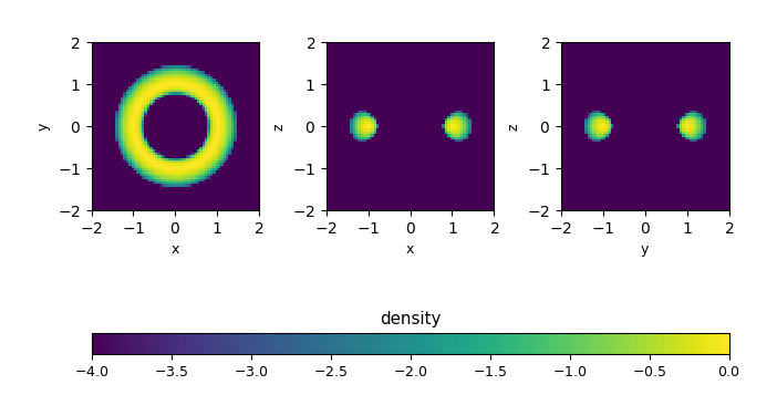
Fig. 2 Initial density (log scale) for the rotating_torus problem with ${64}^3$ zones.

For the standard hydrodynamics algorithm, the torus gets disrupted and spreads out into a disk:

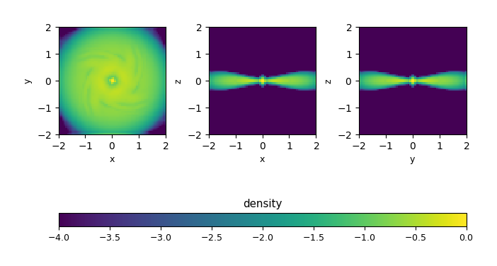
Fig. 3 Density (log scale) for the rotating_torus problem after 200 timesteps, using ${64}^3$ zones. Notice that the initial torus has become disrupted into a disk.

The hybrid momentum algorithm is enabled by setting:

USE_HYBRID_MOMENTUM = TRUE

in your GNUmakefile. With this enabled, we see that the torus remains intact:

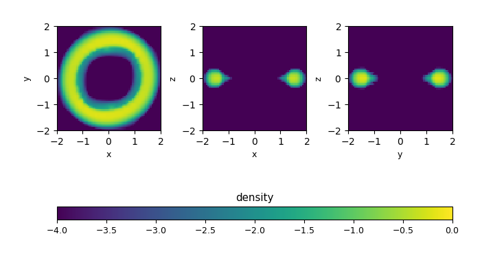
Fig. 4 Density (log scale) for the rotating_torus problem after 200 timesteps with the hybrid momentum algorithm, using ${64}^3$ zones. With this angular-momentum preserving scheme we see that the initial torus is largely intact.