Getting Started
Note
Castro has two source dependencies: AMReX, the adaptive mesh library, and Microphysics, the collection of equations of state, reaction networks, and other microphysics. The instructions below describe how to get these dependencies automatically with Castro.
The compilation process is managed by AMReX and its build system. The general requirements to build Castro are:
A C++20 (or later) compiler (for GCC, we need >= 13.1)
python (>= 3.10)
GNU make (>= 3.82)
GCC is the main compiler suite used by the developers.
For running in parallel, an MPI library is required. For running on GPUs:
CUDA 12 or later is required for NVIDIA GPUs
ROCM 6.3.1 or later is required for AMD GPUs (earlier versions have a register allocation bug)
More information on parallel builds is given in section Running Options: CPUs and GPUs.
Downloading the Code
Castro is maintained as a repository on GitHub, and can be obtained via standard git clone commands. First, make sure that git is installed on your machine—we recommend version 1.7.x or higher.
Clone/fork the Castro repository from the AMReX-Astro GitHub organization, using either HTTP access:
git clone --recursive https://github.com/AMReX-Astro/Castro.gitor SSH access if you have an SSH key enabled with GitHub:
git clone --recursive git@github.com:AMReX-Astro/Castro.gitThe
--recursiveoption togit cloneis used to ensure that all of Castro’s dependencies are downloaded. Currently this requirement is for the AMReX mesh refinement framework, which is maintained in the AMReX-Codes organization on GitHub, and the Microphysics repository from the AMReX-Astro organization. AMReX adds the necessary code for the driver code for the simulation, while Microphysics adds the equations of state, reaction networks, and other microphysics needed to run Castro.If you forget to do a recursive clone, you can rectify the situation by running the following from the top-level of the Castro directory:
git submodule update --init --recursiveNote
By default, you will be on the
mainbranch of the source. Development on Castro (and its primary dependencies, AMReX and Microphysics) is done in thedevelopmentbranch, so you should work there if you want the latest source:git checkout developmentThe Castro team runs nightly regression testing on the
developmentbranch, so bugs are usually found and fixed relatively quickly, but it is generally less stable than staying on themainbranch.We recommend setting the
CASTRO_HOMEenvironment variable to point to the path name where you have put Castro. Add the following to your.bashrc:export CASTRO_HOME="/path/to/Castro/"
(or use the analogous form for a different shell).
You can keep the code up to date with:
git pull --recurse-submodulesThe recommended frequency for doing this is monthly, if you are on the stable
mainbranch of the code; we issue a new release of the code at the beginning of each month.optional, for developers: If you prefer, you can maintain AMReX and Microphysics as standalone repositories rather than as git submodules. To do so, you can clone them from GitHub using:
git clone https://github.com/AMReX-Codes/amrex.git
git clone https://github.com/AMReX-Astro/Microphysics.git
or via SSH as:
git clone git@github.com:/AMReX-Codes/amrex.git
git clone git@github.com:/AMReX-Astro/Microphysics.git
Then, set the
AMREX_HOMEenvironment variable to point to theamrex/directory, and theMICROPHYSICS_HOMEenvironment variable to point to theMicrophysics/directory. Castro will look there instead of in its localexternal/subdirectory.
Building the Code
In Castro each different problem setup is stored in its own
sub-directory under Castro/Exec/. You build the
Castro executable in the problem sub-directory. Here we’ll
build the Sedov problem:
From the directory in which you checked out the Castro git repo, type:
cd Castro/Exec/hydro_tests/SedovThis will put you into a directory in which you can run the Sedov problem in 1-d, 2-d or 3-d.
In
Sedov/, edit theGNUmakefile, and setDIM = 2This is the dimensionality—here we pick 2-d.
COMP = gnuThis is the set of compilers. GNU are a good default choice (this will use g++). You can also choose
intelfor example.If you want to try other compilers than the GNU suite and they don’t work, please let us know.
DEBUG = FALSEThis disables debugging checks and results in a more optimized executable.
USE_MPI = FALSEThis turns off parallelization via MPI. Set it to
TRUEto build with MPI—this requires that you have the MPI library installed on your machine. In this case, the build system will need to know about your MPI installation. This can be done by editing the makefiles in the AMReX tree, but the default fallback is to look for the standard MPI wrappers (e.g.mpic++andmpif90) to do the build.
Now type
make.The resulting executable will look something like
Castro2d.gnu.ex, which means this is a 2-d version of the code compiled withCOMP = gnu.
More information on the various build options is given in Build System Overview.
Running the Code
Castro takes an input file that overrides the runtime parameter defaults. The code is run as:
./Castro2d.gnu.ex inputs.2d.cyl_in_cartcoordsThis will run the 2-d cylindrical Sedov problem in Cartesian (\(x\)-\(y\) coordinates). You can see other possible options, which should be clear by the names of the inputs files.
You will notice that running the code generates directories that look like
plt00000/,plt00020/, etc, andchk00000/,chk00020/, etc. These are “plotfiles” and “checkpoint” files. The plotfiles are used for visualization, the checkpoint files are used for restarting the code.
Visualization of the Results
There are several options for visualizing the data. The popular packages yt and VisIt both support the AMReX file format natively [1]. The standard tool used within the AMReX-community is Amrvis, which we demonstrate here. Amrvis is available on github.
yt
yt is the primary visualization and analysis tool used by the developers. Install yt following their instructions: Getting yt .
You should be able to read in your plotfiles using yt.load() and
do any of the plots described in the yt Cookbook .
Here we do a sample visualization and analysis of the
plotfiles generated. This section was generated from a
Jupyter notebook which can be found in
Docs/source/yt_example.ipynb in the Castro repo.
import yt
import matplotlib.pyplot as plt
import numpy as np

# set matplotlib formatting to be the same as yt
plt.rcParams['font.size'] = 14
plt.rcParams['font.family'] = 'serif'
plt.rcParams['mathtext.fontset'] = 'stix'
# load data from file
ds = yt.load('../../Exec/hydro_tests/Sedov/sedov_2d_cyl_in_cart_plt00150/', hint="castro")
yt : [INFO     ] 2020-05-29 16:40:16,890 Parameters: current_time              = 0.1
yt : [INFO     ] 2020-05-29 16:40:16,891 Parameters: domain_dimensions         = [32 32  1]
yt : [INFO     ] 2020-05-29 16:40:16,891 Parameters: domain_left_edge          = [0. 0. 0.]
yt : [INFO     ] 2020-05-29 16:40:16,892 Parameters: domain_right_edge         = [1. 1. 1.]
# print out fields available for plotting
print([f for _,f in ds.field_list])
['Gamma_1', 'MachNumber', 'StateErr_0', 'StateErr_1', 'StateErr_2', 'Temp', 'X(X)', 'abar', 'angular_momentum_x', 'angular_momentum_y', 'angular_momentum_z', 'circvel', 'density', 'divu', 'eint_E', 'eint_e', 'entropy', 'kineng', 'logden', 'magmom', 'magvel', 'magvort', 'pressure', 'radvel', 'rho_E', 'rho_X', 'rho_e', 'soundspeed', 'x_velocity', 'xmom', 'y_velocity', 'ymom', 'z_velocity', 'zmom']
# plot the density
fig = yt.SlicePlot(ds, 'z', 'density')

# save plot to file
fig.save('sedov_density.png')

fig
yt : [INFO     ] 2020-05-29 16:40:17,234 xlim = 0.000000 1.000000
yt : [INFO     ] 2020-05-29 16:40:17,235 ylim = 0.000000 1.000000
yt : [INFO     ] 2020-05-29 16:40:17,235 xlim = 0.000000 1.000000
yt : [INFO     ] 2020-05-29 16:40:17,236 ylim = 0.000000 1.000000
yt : [INFO     ] 2020-05-29 16:40:17,237 Making a fixed resolution buffer of (('gas', 'density')) 800 by 800
yt : [INFO     ] 2020-05-29 16:40:17,392 Saving plot sedov_density.png

# plot the temperature and annotate the grids
fig = yt.SlicePlot(ds, 'z', 'Temp')
fig.annotate_grids(linewidth=2, alpha=1, edgecolors='red')
fig.annotate_cell_edges(line_width=0.0005, alpha=0.4, color='white')
fig
yt : [INFO     ] 2020-05-29 16:40:17,748 xlim = 0.000000 1.000000
yt : [INFO     ] 2020-05-29 16:40:17,749 ylim = 0.000000 1.000000
yt : [INFO     ] 2020-05-29 16:40:17,750 xlim = 0.000000 1.000000
yt : [INFO     ] 2020-05-29 16:40:17,750 ylim = 0.000000 1.000000
yt : [INFO     ] 2020-05-29 16:40:17,751 Making a fixed resolution buffer of (('boxlib', 'Temp')) 800 by 800
yt : [WARNING  ] 2020-05-29 16:40:17,897 Supplied id_loc but draw_ids is False. Not drawing grid ids
yt : [WARNING  ] 2020-05-29 16:40:17,899 Supplied id_loc but draw_ids is False. Not drawing grid ids
yt : [WARNING  ] 2020-05-29 16:40:17,901 Supplied id_loc but draw_ids is False. Not drawing grid ids
yt : [WARNING  ] 2020-05-29 16:40:17,903 Supplied id_loc but draw_ids is False. Not drawing grid ids
yt : [WARNING  ] 2020-05-29 16:40:17,905 Supplied id_loc but draw_ids is False. Not drawing grid ids
yt : [WARNING  ] 2020-05-29 16:40:17,906 Supplied id_loc but draw_ids is False. Not drawing grid ids
yt : [WARNING  ] 2020-05-29 16:40:17,908 Supplied id_loc but draw_ids is False. Not drawing grid ids
yt : [WARNING  ] 2020-05-29 16:40:17,910 Supplied id_loc but draw_ids is False. Not drawing grid ids
yt : [WARNING  ] 2020-05-29 16:40:17,911 Supplied id_loc but draw_ids is False. Not drawing grid ids

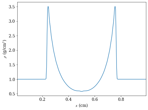
# create a line plot of the density parallel to the x-axis that cuts through the
# point of maximum density

_, c = ds.find_max("density") # find the location of the point of maximum density
ax = 0 # take cut parallel to x-axis

# use ortho_ray to cut through c
ray = ds.ortho_ray(ax, (c[1], c[2]))

# sort values by x so there are no discontinuities in the line plot
srt = np.argsort(ray['x'])

fig, ax = plt.subplots(figsize=(8,6))
ax.plot(ray['x'][srt], ray['density'][srt])
ax.set_xlabel(r'$x$ (cm)')
ax.set_ylabel(r'$\rho$ (g/cm$^3$)')
ax.set_xlim([ray['x'][srt][0], ray['x'][srt][-1]])

fig.savefig('dens_plot.png')
yt : [INFO ] 2020-05-29 16:40:18,254 Max Value is 3.51160e+00 at 0.7558593750000000 0.7558593750000000 0.5000000000000000
Amrvis
Amrvis is a tool developed at LBNL to visualize AMReX data. It provides a simple GUI that allows you to quickly visualize slices and the grid structure.
Get Amrvis:
git clone https://github.com/AMReX-Codes/AmrvisThen cd into
Amrvis/, edit theGNUmakefilethere to setDIM = 2, and again setCOMPto compilers that you have. LeaveDEBUG = FALSE.Type
maketo build, resulting in an executable that looks likeamrvis2d...ex.If you want to build amrvis with
DIM = 3, you must first download and build volpack:git clone https://ccse.lbl.gov/pub/Downloads/volpack.gitThen cd into
volpack/and typemake.Note: Amrvis requires the OSF/Motif libraries and headers. If you don’t have these you will need to install the development version of motif through your package manager. On most Linux distributions, the motif library is provided by the openmotif package, and its header files (like
Xm.h) are provided by openmotif-devel. If those packages are not installed, then use the package management tool to install them, which varies from distribution to distribution, but is straightforward.lesstifgives some functionality and will allow you to build the Amrvis executable, but Amrvis may not run properly.You may then want to create an alias to amrvis2d, for example:
alias amrvis2d=/tmp/Amrvis/amrvis2d...ex
where
/tmp/Amrvis/amrvis2d...exis the full path and name of the Amrvis executable.Configure Amrvis:
Copy the
amrvis.defaultsfile to your home directory (you can rename it to.amrvis.defaultsif you wish). Then edit the file, and change the palette line to point to the full path/filename of thePalettefile that comes with Amrvis.Visualize:
Return to the
Castro/Exec/hydro_tests/Sedovdirectory. You should have a number of output files, including some in the formpltXXXXX, where XXXXX is a number corresponding to the timestep the file was output.amrvis2d filenameto see a single plotfile, oramrvis2d -a plt*, which will animate the sequence of plotfiles.Try playing around with this—you can change which variable you are looking at, select a region and click “Dataset” (under View) in order to look at the actual numbers, etc. You can also export the pictures in several different formats under “File/Export”.
Some users have found that Amrvis does not work properly under X with the proprietary Nvidia graphics driver. A fix for this is provided in the FAQ (§ Runtime Errors)—this is due to the default behavior of the DAC in mappuing colors.