Governing Equations
The equation set and solution procedure used by MAESTROeX has changed and improved over time. In this chapter, we outline the model equations and algorithmic options in the code. The latest published references for MAESTROeX are the multilevel paper [NonakaAlmgrenBell+10] and the more recent [FanNonakaAlmgren+19]. These two papers use the same model equations, however the more recent paper, in addition to retaining the original algorithmic capability of the previous code, includes an option to use a new, simplified temporal integration scheme. We distinguish between the two temporal integration strategies by referring to them as the “original temporal scheme” and “new temporal scheme”. In this description, we make frequent reference to papers I-IV and the multilevel paper (see § Introduction to MAESTROeX), which describe the developments of the original temporal scheme.
Summary of the MAESTROeX Equation Set
Here we summarize the equations solved by MAESTROeX. We refer the reader to papers I through IV for the derivation and motivation of the equation set. We take the standard equations of reacting, compressible flow, and recast the equation of state (EOS) as a divergence constraint on the velocity field. The resulting model is a series of evolution equations for mass, energy, and momentum, subject to an additional constraint on velocity, with a base state density and pressure linked via hydrostatic equilibrium:
We discuss each of these equations in further detail below.
Lateral Average
A key concept in the MAESTROeX equation set and algorithm is the lateral average. The lateral average represents the average value of a quantity at a given radius in spherical simulations (or a given height in planar simulations). We denote the lateral average of a quantity with an overline, e.g., for any quantity \(\phi\), we denote the average of \(\phi\) over a layer at constant radius as \(\overline{\phi}\). For planar problems this routine is a trivial average of all the values at a given height. For spherical problems there is a novel interpolation routine we use to average 3D data representing a full spherical star into a 1D array representing the average. Details can be found in [NonakaAlmgrenBell+10] and [FanNonakaAlmgren+19].
For the velocity field, we can decompose the full velocity field into a base state velocity and a local velocity,
where \(r\) is a 1D radial coordinate, \(\xb\) is a 3D Cartesian grid coordinate, and \(\eb_r\) is the unit vector in the outward radial direction. Note that \(\overline{(\Ubt\cdot\eb_r)} = 0\) and \(w_0 = \overline{(\Ub\cdot\eb_r)}\). In other words, the base state velocity can be thought of as the lateral average of the outward radial velocity. For the velocity decompsotion, we do not use the same spatial averaging operators used for all other variables; instead we derive an analytic expression for the average expansion velocity and numerically integrate this expression to obtain \(w_0\).
Mass
Conservation of mass gives the same continuity equation we have with compressible flow:
where \(\rho\) is the total mass density. Additionally, we model the evolution of individual species that advect and react. The creation and destruction of the species is described by their create rate, \(\omegadot_k\), and the species are defined by their mass fractions, \(X_k \equiv \rho_k / \rho\), giving
and
In the original temporal scheme, we need to model the evolution of a base state density, \(\rho_0\). The governing equation can be obtained by laterally averaging the full continuity equation, giving:
Subtracting these two yields the evolution equation for the perturbational density, \(\rho^\prime \equiv \rho - \rho_0\):
As first discussed in paper III and then refined in the multilevel paper, we capture the changes that can occur due to significant convective overturning by imposing the constraint that \(\overline{\rho'}=0\) for all time. This gives
where
In practice, we correct the drift by simply setting \(\rho_0 = \overline{\rho}\) after the advective update of \(\rho\). However we still need to explicitly compute \(\etarho\) since it appears in other equations.
Energy
We model the evolution of specific enthalpy, \(h\). Strictly speaking this is not necessary to close the system, but a user can enable the option to couple the energy with the rest of the system by using the enthalpy to define the temperature. The advantages of this coupling is an area of active research. The evolution equation is
where \(p_0\) is the 1D base state pressure, \(\Hnuc\) and \(\Hext\) are energy sources due to reactions and user-defined external heating.
When we are using thermal diffusion, there will be an additional term in the enthalpy equation (see § Thermal Diffusion Changes).
In the original temporal scheme, we utilized a base state enthlpy that effectively represents the average over a layer; its evolution equation can be found by laterally averaging Eq.27
We will often expand \(Dp_0/Dt\) as
where we defined
In paper III, we showed that for a plane-parallel atmosphere with constant gravity, \(\psi = \etarho g\)
At times, we will define a temperature equation by writing \(h = h(T,p,X_k)\) and differentiating:
Subtracting it from the full enthalpy equation gives:
Base State
The stratified atmosphere is characterized by a one-dimensional time-dependent base state, defined by a base state density, \(\rho_0\), and a base state pressure, \(p_0\), in hydrostatic equilibrium:
The gravitational acceleration, \(g\) is either constant or a point-mass with a \(1/r^2\) dependence (see § Modifications for a 1/r^2 Plane-Parallel Basestate) for plane-parallel geometries, or a monopole constructed by integrating the base state density for spherical geometries.
For the time-dependence, we will define a base state velocity, \(w_0\), which will adjust the base state from one hydrostatic equilibrium to another in response to heating.
For convenience, we define a base state enthalphy, \(h_0\), as needed by laterally averaging the full enthalpy, \(h\).
Base State Expansion
In practice, we calculate \(w_0\) by integrating the one-dimensional divergence constraint. For a plane-parallel atmosphere, the evolution is:
Then we define
once \(w_0\) at the old and new times is known, and the advective term is computed explicitly. Then we can include this for completeness in the update for \(\ut.\)
Momentum
The compressible momentum equation (written in terms of velocity is):
Subtracting off the equation of hydrostatic equilibrium, and defining the perturbational pressure (sometimes called the dynamic pressure) as \(\pi \equiv p - p_0\), and perturbational density as \(\rho' \equiv \rho - \rho_0\), we have:
or
This is the form of the momentum equation that we solved in papers I–IV and in the multilevel paper.
Several authors [KP12, VLB+13] explored the idea of energy conservation in a low Mach number system and found that an additional term (which can look like a buoyancy) is needed in the low Mach number formulation, yielding:
This is the form that we enforce in MAESTROeX, and the choice is controlled
by use_alt_energy_fix.
We decompose the full velocity field into a base state velocity, \(w_0\), that governs the base state dynamics, and a local velocity, \(\Ubt\), that governs the local dynamics, i.e.,
with \(\overline{(\Ubt\cdot\eb_r)} = 0\) and \(w_0 = \overline{(\Ub\cdot\eb_r)}\)—the motivation for this splitting was given in paper II. The velocity evolution equations are then
where \(\pi_0\) is the base state component of the perturbational pressure. By laterally averaging to Eq.45, we obtain a divergence constraint for \(w_0\):
The divergence constraint for \(\Ubt\) can be found by subtracting Eq.43 into Eq.45, resulting in
Velocity Constraint
The equation of state is cast into an elliptic constraint on the velocity field by differentiating \(p_0(\rho, s, X_k)\) along particle paths, giving:
where \(\beta_0\) is a density-like variable that carries background stratification, defined as
and
where \(p_{X_k} \equiv \left. \partial p / \partial X_k
\right|_{\rho,T,X_{j,j\ne k}}\), \(\xi_k \equiv \left. \partial h /
\partial X_k \right |_{p,T,X_{j,j\ne k}},
p_\rho \equiv \left. \partial p/\partial \rho \right |_{T, X_k}\), and
\(\sigma \equiv p_T/(\rho c_p p_\rho)\), with
\(p_T \equiv \left. \partial p / \partial T \right|_{\rho, X_k}\) and
\(c_p \equiv \left. \partial h / \partial T
\right|_{p,X_k}\) is the specific heat at constant pressure. The last
term is only present if we are using thermal diffusion (use_thermal_diffusion = T). In this term, \(\kth\) is the thermal conductivity.
In this constraint, \(\gammabar\) is the lateral average of \(\Gamma_1 \equiv d\log p / d\log \rho |_s\). Using the lateral average here makes it possible to cast the constraint as a divergence. [KP12] discuss the general case where we want to keep the local variations of \(\Gamma_1\) (and we explored this in paper III). We also look at this in § \Gamma_1 Variation Changes
Notation
Throughout the papers describing MAESTROeX, we’ve largely kept our notation consistent. The table below defines the frequently-used quantities and provides their units.
symbol |
description |
units |
|---|---|---|
\(c_p\) |
specific heat at constant pressure (\(c_p \equiv \partial h / \partial T |_{p, X_k}\)) |
erg g \(^{-1}\) K \(^{-1}\) |
\(f\) |
volume discrepancy factor (\(0 \le f \le 1\)) |
– |
\(g\) |
gravitational acceleration |
cm s \(^{-2}\) |
\(h\) |
specific enthalpy |
erg g \(^{-1}\) |
\(\Hext\) |
external heating energy generation rate |
erg g \(^{-1}\) s \(^{-1}\) |
\(\Hnuc\) |
nuclear energy generation rate |
erg g \(^{-1}\) s \(^{-1}\) |
\(h_p\) |
\(h_p \equiv \partial h/\partial p |_{T,X_k}\) |
cm \(^{3}\) g \(^{-1}\) |
\(\kth\) |
thermal conductivity |
erg cm \(^{-1}\) s \(^{-1}\) K \(^{-1}\) |
\(p_0\) |
base state pressure |
erg cm \(^{-3}\) |
\(p_T\) |
\(p_T \equiv \partial p / \partial T |_{\rho,X_k}\) |
erg cm \(^{-3}\) K \(^{-1}\) |
\(p_{X_k}\) |
\(p_{X_k}\equiv\partial p/\partial X_k|_{p,T,X_{j,j\ne k}}\) |
erg cm \(^{-3}\) |
\(p_\rho\) |
\(p_\rho \equiv \partial p/\partial \rho |_{T,X_k}\) |
erg g \(^{-1}\) |
\(q_k\) |
specific nuclear binding energy |
erg g\(^{-1}\) |
\(r\) |
radial coordinate (direction of gravity) |
cm |
\(s\) |
specific entropy |
erg g \(^{-1}\) K \(^{-1}\) |
\(S\) |
source term to the divergence constraint |
s \(^{-1}\) |
\(t\) |
time |
s |
\(T\) |
temperature |
K |
\(\Ub\) |
total velocity (\(\Ub = \Ubt + w_0 \eb_r\) |
cm s \(^{-1}\) |
\(\Ubt\) |
local velocity |
cm s \(^{-1}\) |
\(\uadv\) |
advective velocity (edge-centered) |
cm s \(^{-1}\) |
\(w_0\) |
base state expansion velocity |
cm s\(^{-1}\) |
\(X_k\) |
mass fraction of the species (\(\sum_k X_k = 1\)) |
– |
\(\beta_0\) |
coefficient to velocity in velocity constraint equation |
g cm \(^{-3}\) |
\(\Gamma_1\) |
first adiabatic exponent (\(\Gamma_1 \equiv d\log p/d\log \rho|_s\)) |
– |
\(\etarho\) |
\(\etarho \equiv \overline{(\rho' \Ub \cdot \eb_r)}\) |
g cm \(^{-2}\) s \(^{-1}\) |
\(\xi_k\) |
\(\xi_k \equiv \partial h / \partial X_k |_{p,T,X_{j,j\ne k}}\) |
erg g \(^{-1}\) |
\(\pi\) |
dynamic pressure |
erg cm \(^{-3}\) |
\(\pizero\) |
base state dynamic pressure |
erg cm \(^{-3}\) |
\(\rho\) |
mass density |
g cm \(^{-3}\) |
\(\rho_0\) |
base state mass density |
g cm \(^{-3}\) |
\(\rho'\) |
perturbational density (\(\rho' = \rho - \rho_0\)) |
g cm \(^{-3}\) |
\((\rho h)_0\) |
base state enthalpy density |
erg cm \(^{-3}\) |
\((\rho h)'\) |
perturbational enthalpy density \(\left [(\rho h)' = \rho h - (\rho h)_0 \right ]\) |
erg cm \(^{-3}\) |
\(\sigma\) |
\(\sigma \equiv p_T/(\rho c_p p_\rho)\) |
erg \(^{-1}\) g |
\(\psi\) |
\(\psi \equiv D_0 p_0/Dt = \ptl p_0/\ptl t + w_0\ptl p_0/\ptl r\) |
erg cm \(^{-3}\) |
\(\omegadot_k\) |
creation rate for species \(k\) (\(\omegadot_k \equiv DX_k/Dt\)) |
s \(^{-1}\) |
Time Advancement Algorithm Ingredients
The full time advancement algorithm is detailed in [NonakaAlmgrenBell+10] for the original algorithm and [FanNonakaAlmgren+19] for the new, simplified algorithm. We do not repeat that here.
The overall flow of the algorithm is depicted in the following flowcharts:
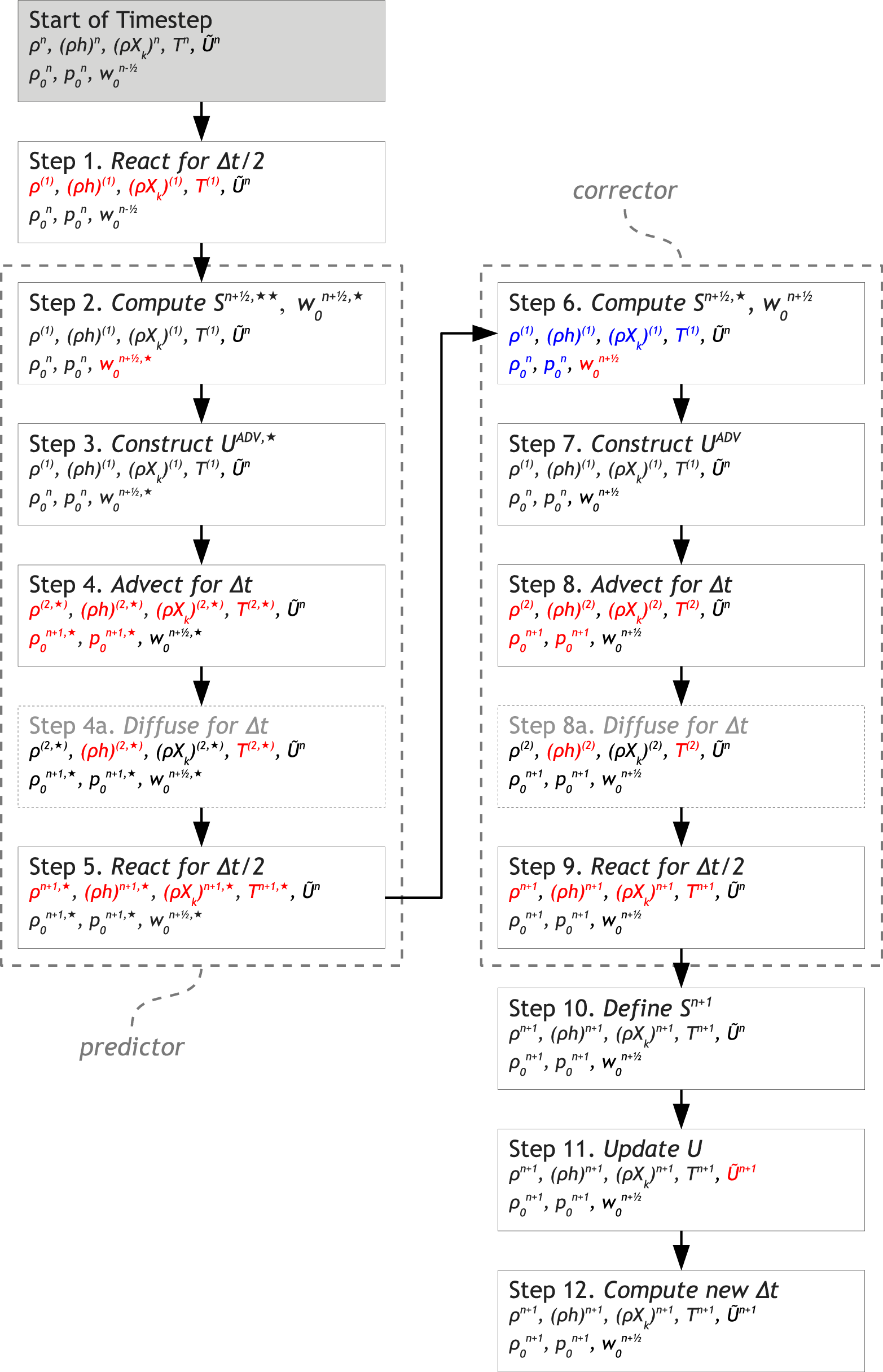
Fig. 1 A flowchart of the algorithm. The thermodynamic state variables, base state variables, and local velocity are indicated in each step. Red text indicates that quantity was updated during that step. The predictor-corrector steps are outlined by the dotted box. The blue text indicates state variables that are the same in Step 6 as they are in Step 2, i.e., they are unchanged by the predictor steps. The diffusion steps (4a and 8a) are optional, depending on use_thermal_diffusion.
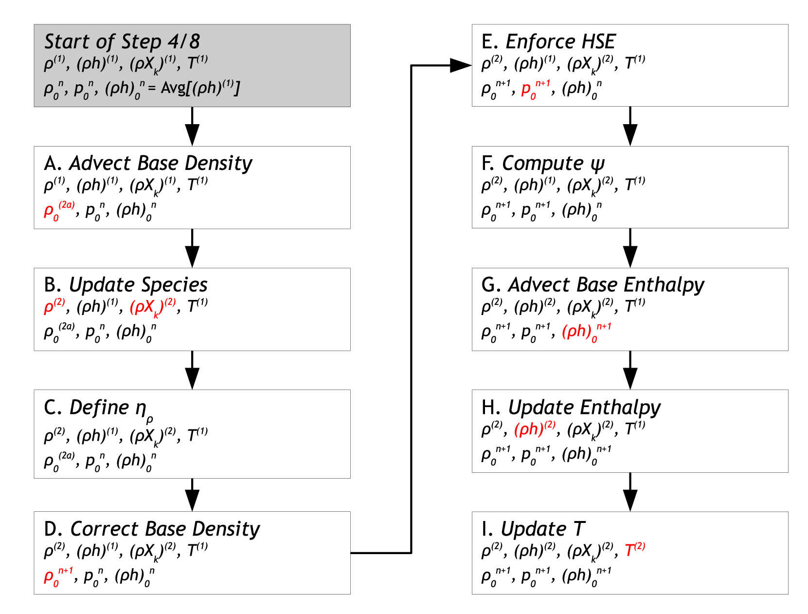
Fig. 2 A flowchart for Steps 4 and 8. The thermodynamic state variables and base state variables are indicated in each step. Red text indicates that quantity was updated during that step. Note, for Step 4, the updated quantities should also have a \(⋆\) superscript, e.g., Step 8I defines \(T^{(2)}\) while Step 4I defines \(T^{(2),\star}\).
Here are some of the basic ingredients to the solver:
Definitions
Below we define operations that will be referenced in § Volume Discrepancy Changes.
React State\([\rho^{\inp},(\rho h)^{\inp},X_k^{\inp},T^{\inp}, (\rho\Hext)^{\inp}, p_0^{\inp}] \rightarrow [\rho^{\outp}, (\rho h)^{\outp}, X_k^{\outp}, T^{\outp}, (\rho \omegadot_k)^{\outp}, (\rho\Hnuc)^{\outp}]\) evolves the species and enthalpy due to reactions through \(\Delta t/2\) according to:
Here the temperature equation comes from Eq.31 with \(Dp_0/Dt = 0\) for the burning part of the evolution.
Full details of the solution procedure can be found in Paper III. We then define:
where the enthalpy update includes external heat sources \((\rho\Hext)^{\inp}\). As introduced in Paper IV, we update the temperature using \(T^{\outp} = T(\rho^\outp,h^\outp,X_k^\outp)\) for planar geometry or \(T^{\outp} = T(\rho^\outp,p_0^\inp,X_k^\outp)\) for spherical geometry, with this behavior controlled by use_tfromp. Note that the density remains unchanged within React State, i.e., \(\rho^{\outp} = \rho^{\inp}\).
The source code for this operation can be found in react_state.f90.
Advect Base Density
\([\rho_0^\inp,w_0^\inp] \rightarrow [\rho_0^\outp, \rho_0^{\outp,\nph}]\) is the process by which we update the base state density through \(\dt\) in time. We keep the time-centered edge states, \(\rho_0^{\outp,\nph}\), since they are used later in discretization of \(\etarho\) for planar problems.
planar:
We discretize equation Eq.23 to compute the new base state density,
(50)\[\rho_{0,j}^{\outp} = \rho_{0,j}^{\inp} - \frac{\dt}{\dr} \left [ \left( \rho_0^{\outp,\nph} w_0^{\inp}\right)_{j+\myhalf} - \left( \rho_0^{\outp,\nph} w_0^{\inp}\right)_{j-\myhalf} \right ].\]We compute the time-centered edge states, \({\rho_0}^{\outp,\nph}_{j\pm\myhalf}\), by discretizing an expanded form of Eq.23:
(51)\[\frac{\partial \rho_0}{\partial t} + w_0 \frac{\partial \rho_0}{\partial r} = - \rho_0 \frac{\partial w_0}{\partial r},\]where the right hand side is used as the force term.
spherical:
The base state density update now includes the area factors in the divergences:
(52)\[\rho_{0,j}^{\outp} = \rho_{0,j}^{\inp} - \frac{1}{r_j^2} \frac{\dt}{\dr} \left [ \left( r^2 \rho_0^{\outp,\nph} w_0^{\inp}\right)_{j+\myhalf} - \left( r^2 \rho_0^{\outp,\nph} w_0^{\inp}\right)_{j-\myhalf} \right].\]In order to compute the time-centered edge states, an additional geometric term is added to the forcing, due to the spherical discretization of Eq.23:
(53)\[\frac{\partial \rho_0}{\partial t} + w_0 \frac{\partial \rho_0}{\partial r} = - \rho_0 \frac{\partial w_0}{\partial r} - \frac{2 \rho_0 w_0}{r}.\]
Enforce HSE
\([p_0^{\inp},\rho_0^{\inp}] \rightarrow [p_0^{\outp}]\) has replaced Advect Base Pressure from Paper III as the process by which we update the base state pressure. Rather than discretizing the evolution equation for \(p_0\), we enforce hydrostatic equilibrium directly, which is numerically simpler and analytically equivalent. We first set \(p_{0,j=0}^{\outp} = p_{0,j=0}^{\inp}\) and then update \(p_0^\outp\) using:
where \(g=g(\rho_0^\inp)\). As soon as \(\rho_{0,j}^\inp < \rho_{\rm cutoff}\), we set \(p_{0,j+1}^\outp = p_{0,j}^\outp\) for all remaining values of \(j\). Then we compare \(p_{0,j_{\rm max}}^\outp\) with \(p_{0,j_{\rm max}}^\inp\) and offset every element in \(p_0^\outp\) so that \(p_{0,j_{\rm max}}^\outp = p_{0,j_{\rm max}}^\inp\). We are effectively using the location where the \(\rho_0^\inp\) drops below \(\rho_{\rm cutoff}\) as the starting point for integration.
Advect Base Enthalpy
\([(\rho h)_0^\inp,w_0^\inp,\psi^\inp] \rightarrow [(\rho h)_0^\outp]\) is the process by which we update the base state enthalpy through \(\dt\) in time.
planar:
We discretize Eq.28, neglecting reaction source terms, to compute the new base state enthalpy,
(55)\[(\rho h)_{0,j}^{\outp} = (\rho h)_{0,j}^{\inp} - \frac{\dt}{\Delta r} \left\{ \left[ (\rho h)_0^{\nph} w_0^{\inp}\right]_{j+\myhalf} - \left[ (\rho h)_0^{\nph} w_0^{\inp}\right]_{j-\myhalf} \right\} + \dt\psi_j^{\inp}.\]We compute the time-centered edge states, \((\rho h)_0^{\nph}\), by discretizing an expanded form of Eq.28:
(56)\[\frac{\partial (\rho h)_0}{\partial t} + w_0 \frac{\partial (\rho h)_0}{\partial r} = -(\rho h)_0 \frac{\partial w_0}{\partial r} + \psi.\]spherical:
The base state enthalpy update now includes the area factors in the divergences:
(57)\[\begin{split}\begin{aligned} (\rho h)_{0,j}^{\outp} &= (\rho h)_{0,j}^{\inp} \nonumber \\ & - \frac{1}{r_j^2} \frac{\dt}{\dr} \left \{ \left[ r^2 (\rho h)_0^{\nph} w_0^{\inp}\right]_{j+\myhalf} - \left[ r^2 (\rho h)_0^{\nph} w_0^{\inp}\right]_{j-\myhalf} \right\} +\dt\psi^{\inp,\nph}.\nonumber\\\end{aligned}\end{split}\]In order to compute the time-centered edge states, an additional geometric term is added to the forcing, due to the spherical discretization of Eq.28:
(58)\[\frac{\partial (\rho h)_0}{\partial t} + w_0 \frac{\partial (\rho h)_0}{\partial r} = -(\rho h)_0 \frac{\partial w_0}{\partial r} - \frac{2 (\rho h)_0 w_0}{r} + \psi.\]
Computing \(w_0\)
Here we describe the process by which we compute \(w_0\). The arguments are different for planar and spherical geometries.
planar:
\([\Sbar^{\inp},\gammabar^{\inp}, p_0^{\inp},\psi^{\inp}]\rightarrow [w_0^{\outp}]\):
In Paper III, we showed that \(\psi=\etarho g\) for planar geometries, and derived derived Eq.34 as an alternate expression for eq:eq:w0 divergence. We discretize this as:
(59)\[\frac{w_{0,j+\myhalf}^\outp-w_{0,j-\myhalf}^\outp}{\Delta r} = \left(\Sbar^{\inp} - \frac{1}{\gammabar^{\inp} p_0^{\inp}}\psi^{\inp}\right)_j,\]with \(w_{0,-\myhalf}=0\).
spherical:
\([\Sbar^{\inp},\gammabar^{\inp},\rho_0^{\inp},p_0^{\inp},\etarho^{\inp}] \rightarrow[w_0^{\outp}]\):
We begin with Eq.43 written in spherical coordinates:
(60)\[\frac{1}{r^2}\frac{\partial}{\partial r} \left (r^2 \beta_0 w_0 \right ) = \beta_0 \left ( \Sbar - \frac{1}{\gammabar p_0} \frac{\partial p_0}{\partial t} \right ).\]We expand the spatial derivative and recall from Paper I that
(61)\[\frac{1}{\gammabar p_0} \frac{\partial p_0}{\partial r} = \frac{1}{\beta_0} \frac{\partial \beta_0}{\partial r},\]giving:
(62)\[\frac{1}{r^2} \frac{\partial}{\partial r} \left (r^2 w_0 \right ) = \Sbar - \frac{1}{\gammabar p_0} \underbrace{\left( \frac{\partial p_0}{\partial t} + w_0 \frac{\partial p_0}{\partial r} \right)}_{\psi} .\]We solve this equation for \(w_0\) as described in Appendix B of the multilevel paper.
Volume Discrepancy Changes
Chapter [ch:volume] describes the reasoning behind the volume discrepancy term—a forcing term added to the constraint equation to bring us back to the equation of state. This addition of this term (enabled with dpdt_factor= T) modifies our equation set in the following way:
In Step 2B, to compute \(w_0\), we need to account for the volume discrepancy term by first defining \(p_{\rm EOS}^n = \overline{p(\rho,h,X_k)^n}\), and then using:
(63)\[\frac{\partial w_0^{\nph,\star}}{\partial r} = \overline{S^{\nph,\star\star}} - \frac{1}{\overline{\Gamma_1^n}p_0^n}\psi^{\nmh} - \underbrace{\frac{f}{\overline{\Gamma_1^n}p_0^n}\left(\frac{p_0^n-\overline{p_{\rm EOS}^n}}{\Delta t}\right)}_{\delta\chi_{w_0}}.\]In Step 3, the MAC projection should account for the volume discrepancy term:
(64)\[\nabla \cdot \left(\beta_0^n \uadvone\right) = \beta_0^n \left[ \left(S^{\nph,\star\star} - \overline{S^{\nph,\star\star}}\right) + \underbrace{\frac{f}{\gammabar^n p_0^n} \left(\frac{p_{\rm EOS}^n - \overline{p_{\rm EOS}^n}}{\Delta t^n}\right)}_{\delta\chi}\right].\]In Step 6B, to compute \(w_0\), we need to account for the volume discrepancy term by first defining \(p_{\rm EOS}^{n+1,\star} = p(\rho,h,X_k)^{n+1,\star}\), \(\overline{\Gamma_1^{\nph,\star}} = (\overline{\Gamma_1^{n}}+\overline{\Gamma_1^{n+1,\star}})/2\), and \(p^{\nph,\star} = (p^{n}+p^{n+1,\star})/2\), and then using:
(65)\[\frac{\partial w_0^{\nph}}{\partial r} = \overline{S^{\nph,\star}} - \frac{1}{\overline{\Gamma_1^{\nph,\star}}p_0^{\nph,\star}}\psi^{\nph,\star} - \frac{f}{\overline{\Gamma_1^{n+1,\star}}p_0^{n+1,\star}}\left(\frac{p_0^{n+1,\star}-\overline{p_{\rm EOS}^{n+1,\star}}}{\Delta t}\right) - \delta\chi_{w_0}\]In Step 7, the MAC projection should account for the volume discrepancy term:
(66)\[\nabla \cdot \left(\beta_0^{\nph,\star} \uadvtwo\right) = \beta_0^{\nph,\star}\left[\left(S^{\nph,\star} - \overline{S^{\nph,\star}}\right) + \frac{f}{\overline{\Gamma_1^{n+1,\star}} p_0^{n+1,\star}} \left(\frac{p_{\rm EOS}^{n+1,\star} - \overline{p_{\rm EOS}^{n+1,\star}}}{\Delta t^n}\right) + \delta\chi\right],\]where \(p(\rho,h,X_k)^{\nph,\star} = \left[p(\rho,h,X_k)^n +p(\rho,h,X_k)^{n+1,\star}\right]/2\).
In Step 11, the approximate projection should account for the volume discrepancy term:
(67)\[\nabla \cdot \left(\beta_0^{\nph} \Ubt^{n+1} \right) = \beta_0^{\nph}\left\{ \left(S^{n+1} - \overline{S^{n+1}} \right) + \frac{f}{\overline{\Gamma_1^{n+1}} p_0^{n+1}} \left[\frac{p(\rho,h,X_k)^{n+1} - \overline{p(\rho,h,X_k)^{n+1}}}{\Delta t^n}\right]\right\}.\]
\(\Gamma_1\) Variation Changes
The constraint we derive from requiring the pressure to be close to the background hydrostatic pressure takes the form:
The default MAESTROeX algorithm replaces \(\Gamma_1\) with \(\gammabar\), allowing us to write this as a divergence constraint. In paper III, we explored the effects of localized variations in \(\Gamma_1\) by writing \(\Gamma_1 = \gammabar + \delta \Gamma_1\). This gives us:
Assuming that \(\delta \Gamma_1 \ll \gammabar\), we then have
Grouping by order of the correction, we have
Keeping to First Order in \(\delta\Gamma_1\)
The base state evolution equation is the average of Eq.71 over a layer
where we see that the \([\delta \Gamma_1/(\Gamma_1^2 p_0)] \partial p_0/\partial t\) terms averages to zero, since the average of \(\delta\Gamma_1\) term is zero. Subtracting this from Eq.71, we have
These can be written more compactly as:
for plane-parallel geometries (analogous to Eq.34, and
This constraint is not in a form that can be projected. To solve this form, we need to use a lagged \(\Ubt\) in the righthand side.
This change comes into MAESTROeX in a variety of steps, summarized here. To enable this portion of the algorithm, set use_delta_gamma1_term = T.
In Step 3, we are doing the “predictor” portion of the MAESTROeX algorithm, getting the MAC velocity that satisfies the constraint, so we do not try to incorporate the \(\delta \Gamma_1\) effect. We set all the \(\delta \Gamma_1\) terms in Eq.75 to zero.
In Step 6, we are computing the new time-centered source, \(S^{\nph,\star}\) and the base state velocity, \(w_0^\nph\). Now we can incorporate the \(\delta \Gamma_1\) effect. First we construct:
(76)\[\frac{\delta \Gamma_1}{\Gamma_1^2 p_0} \Ubt \cdotb \nablab p_0 \approx \frac{\Gamma_1^{n+1,\star} - \overline{\Gamma_1^{n+1,\star}}} {{\overline{\Gamma_1^{n+1,\star}}}^2} \frac{1}{p_0^n} \Ubt^n \cdotb \nablab p_0^n\]Then we call average to construct the lateral average of this
(77)\[\overline{\frac{\delta \Gamma_1}{\Gamma_1^2 p_0} \Ubt \cdotb \nablab p_0} = \mathbf{Avg} \left (\frac{\Gamma_1^{n+1,\star} - \overline{\Gamma_1^{n+1,\star}}} {{\overline{\Gamma_1^{n+1,\star}}}^2} \frac{1}{p_0^n} \Ubt^n \cdotb \nablab p_0^n \right )\]Since the average of this is needed in advancing \(w_0\), we modify \(\overline{S}\) to include this average:
(78)\[\overline{S^{\nph,\star}} \leftarrow \overline{S^{\nph,\star}} + \overline{\frac{\delta \Gamma_1}{\Gamma_1^2 p_0} \Ubt \cdotb \nablab p_0}\]In Step 7, we now include the \(\delta \Gamma_1\) term in the righthand side for the constraint by solving:
(79)\[\nabla \cdot \left(\beta_0^{\nph,\star} \uadvtwo\right) = \beta_0^{\nph,\star}\left( S^{\nph,\star} - \overline{S^{\nph,\star}} + \frac{\Gamma_1^{n+1,\star} - \overline{\Gamma_1^{n+1,\star}}} {{\overline{\Gamma_1^{n+1,\star}}}^2} \frac{1}{p_0^n} (\psi^{\nph,\star} + \Ubt^n \cdotb \nablab p_0^n) \right)\]We note that this includes the average of the correction term as shown in Eq.75 because we modified \(\bar{S}\) to include this already.
In Step 10, we do a construction much like that done in Step 6, but with the time-centerings of some of the quantities changed. First we construct:
(80)\[\frac{\delta \Gamma_1}{\Gamma_1^2 p_0} \Ubt \cdotb \nablab p_0 \approx \frac{\Gamma_1^{n+1} - \overline{\Gamma_1^{n+1}}} {{\overline{\Gamma_1^{n+1}}}^2} \frac{1}{p_0^{n+1}} \Ubt^n \cdotb \nablab p_0^{n+1}\]Then we call average to construct the lateral average of this
(81)\[\overline{\frac{\delta \Gamma_1}{\Gamma_1^2 p_0} \Ubt \cdotb \nablab p_0} = \mathbf{Avg} \left (\frac{\Gamma_1^{n+1} - \overline{\Gamma_1^{n+1}}} {{\overline{\Gamma_1^{n+1}}}^2} \frac{1}{p_0^{n+1}} \Ubt^n \cdotb \nablab p_0^{n+1} \right )\]Again we modify \(\overline{S}\) to include this average:
(82)\[\overline{S^{n+1}} \leftarrow \overline{S^{n+1}} + \overline{\frac{\delta \Gamma_1}{\Gamma_1^2 p_0} \Ubt \cdotb \nablab p_0}\]In Step 11, we modify the source of the constraint to include the \(\delta \Gamma_1\) information. In particular, we solve:
(83)\[\nabla \cdot \left(\beta_0^{\nph} \Ubt^{n+1} \right) = \beta_0^{\nph} \left(S^{n+1} - \overline{S^{n+1}} + \frac{\Gamma_1^{n+1} - \overline{\Gamma_1^{n+1}}} {{\overline{\Gamma_1^{n+1}}}^2} \frac{1}{p_0^{n+1}} (\psi^{\nph} + \Ubt^n \cdotb \nablab p_0^{n+1}) \right)\]
Thermal Diffusion Changes
Thermal diffusion was introduced in the XRB [MaloneNonakaAlmgren+11]. This introduces a new term to \(S\) as well as the enthalpy equation. Treating the enthalpy equation now requires a parabolic solve. We describe that process here.
Immediately after Step 4H, diffuse the enthalpy through a time interval of \(\dt\). First, define \((\rho h)^{(1a),\star} = (\rho h)^{(2),\star}\). We recompute \((\rho h)^{(2),\star}\) to account for thermal diffusion. Here we begin with the enthalpy equation, but consider only the diffusion terms,
We can recast this as an enthalpy-diffusion equation by applying the chain-rule to \(h(p_0,T,X_k)\),
giving
Compute \(\kth^{(1)}, c_p^{(1)}\), and \(\xi_k^{(1)}\) from \(\rho^{(1)}, T^{(1)}\), and \(X_k^{(1)}\) as inputs to the equation of state. The update is given by
which is numerically implemented as a diffusion equation for \(h^{(2),\star}\),
Immediately after Step 8H, diffuse the enthalpy through a time interval of \(\dt\). First, define \((\rho h)^{(1a)} = (\rho h)^{(2)}\). We recompute \((\rho h)^{(2)}\) to account for thermal diffusion. Compute \(\kth^{(2),\star}, c_p^{(2),\star}\), and \(\xi_k^{(2),\star}\), from \(\rho^{(2),\star}, T^{(2),\star}\), and \(X_k^{(2),\star}\) as inputs to the equation of state. The update is given by
which is numerically implemented as a diffusion equation for \(h^{(2)}\).
Initialization
We start each calculation with user-specified initial values for \(\rho\), \(X_k\) and \(T,\) as well as an initial background state. In order for the low Mach number assumption to hold, the initial data must be thermodynamically consistent with the initial background state. In addition, the initial velocity field must satisfy an initial approximation to the divergence constraint. We use an iterative procedure to compute both an initial right-hand-side for the constraint equation and an initial velocity field that satisfies the constraint. The user specifies the number of iterations, \(N_{\rm iters}^{S},\) in this first step of the initialization procedure.
First, we need to construct approximations to \(S^0, w_0^{-\myhalf}, \Delta t^0\), and \(\Ub^0\). Start with initial data \(X_k^{\initp}, \rho^{\initp},\) \(T^{\initp},\) an initial base state, and an initial guess for the velocity, \(\Ub^{\initp}\). Set \(w_0^0 = 0\) as an initial approximation. Use the equation of state to determine \((\rho h)^{\initp}\). Compute \(\beta_0^0\) as a function of the initial data. The next part of the initialization process proceeds as follows.
Initial Projection: if
do_initial_projection = T, then we first project the velocity field with \(\rho = 1\) and \(\beta_0^0\). The initial projection does not see reactions or external heating, and thus we set \(\dot\omega = \Hnuc = \Hext = 0\) in \(S\). The reason for ignoring reactions and heating is that we need some kind of time scale over which to compute the effect of reactions, but we first need an estimate of the velocity field in order to derive the time step that will be used as a time scale. The elliptic equation we solve is(91)\[\nabla \cdot \beta_0^0 \nabla \phi = \underbrace{\beta_0^0(S - \Sbar)}_\mathrm{0~ except~ for~ diffusion} - \nabla \cdot (\beta_0^0 \Ub^{\initp})\]This \(\phi\) is then used to correct the velocity field to obtain \(\Ub^{0,0}\). If do_initial_projection = F, set \(\Ub^{0,0} = \Ub^{\initp}\).
“Divu” iterations: Next we do
init_divu_iteriterations to project the velocity field using a constraint that sees reactions and external heating. The initial timestep estimate is provided byfirstdtand \(\Ub^{0,0}\), to allow us to compute the effect of reactions over \(\Delta t/2\).Do \(\nu = 1,...,N_{\rm iters}^{S}\).
Estimate \(\Delta t^\nu\) using \(\Ub^{0,\nu-1}\) and \(w_0^{\nu-1}.\)
React State\([ \rho^{\initp},(\rho h)^{\initp}, X_k^{\initp}, T^{\initp}, (\rho^{\initp} \Hext), p_0^{\initp}] \rightarrow [\rho^{\outp}, (\rho h)^{\outp}, X_k^{\outp}, T^{\outp}, (\rho \omegadot_k)^{0,\nu} ].\)
Compute \(S^{0,\nu}\) using \((\rho \omegadot_k)^{0,\nu}\) and the initial data.
Compute \(\overline{S^{0,\nu}} = {\mathrm{\bf Avg}} (S^{0,\nu}).\)
Compute \(w_0^{\nu}\) as in Step 2B using \(\overline{S^{0,\nu}}\) and \(\psi=0\).
Project \(\Ub^{0,\nu-1}\) using \(\beta_0^0\) and \((S^{0,\nu} - \overline{S^{0,\nu}})\) as the source term. This yields \(\Ub^{0,\nu}.\) In this projection, again the density is set to 1, and the elliptic equation we solve is:
(92)\[\nabla \cdot \beta_0^0 \nabla \phi = \beta_0 (S - \Sbar)- \nabla \cdot (\beta_0^0 \Ub^{0,\nu-1})\]
End do.
Define \(S^0 = S^{0,N_{\rm iters}^S}\), \(w_0^{-\myhalf} = w_0^{N_{\rm iters}^S}\), \(\dt^0 = \Delta t^{N_{\rm iters}^S},\) and \(\Ub^0 = \Ub^{0,N_{\rm iters}^S}.\)
Next, we need to construct approximations to \(\etarho^{-\myhalf}, \psi^{-\myhalf}, S^1\), and \(\pi^{-\myhalf}\). As initial approximations, set \(\etarho^{-\myhalf}=0, \psi^{-\myhalf}=0, S^{1,0}=S^0\), and \(\pi^{-\myhalf}=0.\)
Pressure iterations: Here we do
init_iteriterations to get an approximation for the lagged pressure:Do \(\nu = 1,...,N_{\rm iters}^{\pi}\).
Perform Steps 1-11 as described above, using \(S^{\myhalf,\star\star} = (S^0 + S^{1,\nu-1})/2\) in Step 2 as described. The only other difference in the time advancement is that in Step 11 we define \({\bf V} = (\Ubt^{1,\star} - \Ubt^0)\) and solve
(93)\[L_\beta^\rho \phi = D \left ( \beta_0^{\myhalf} {\bf V} \right) - \beta_0^{\myhalf} \left[ \left(S^{1}-\overline{S^{1}}\right) - \left(S^{0}-\overline{S^{0}}\right) \right] .\](The motivation for this form of the projection in the initial pressure iterations is discussed in [ABC00].) We discard the new velocity resulting from this, but keep the new value for \(\pi^{\myhalf} = \pi^{-\myhalf} + (1 / \dt) \; \phi.\) These steps also yield new scalar data at time \(\dt,\) which we discard, and new values for \(\etarho^{\myhalf}\) (Step 8C), \(\psi^{\myhalf}\) (Step 8F), \(S^{1,\nu}\) (Step 10A), and \(\pi^{\myhalf}\) (Step 11), which we keep.
Set \(\pi^{-\myhalf} = \pi^{\myhalf}\), \(\etarho^{-\myhalf} = \etarho^{\myhalf}\), and \(\psi^{-\myhalf} = \psi^{\myhalf}\).
End do.
Finally, we define \(S^1 = S^{1,N_{\rm iters}^\pi}.\)
The tolerances for these elliptic solves are described in § Multigrid.
Changes from Earlier Implementations
Changes Between Paper 3 and Paper 4
We defined the mapping of data between a 1D radial array and the 3D Cartesian grid for spherical problems (which we improve upon in the multilevel paper).
We update \(T\) after the call to React State.
We have created a burning_cutoff_density, where the burning does not happen below this density. It is presently set to
base_cutoff_density.Use corner coupling in advection.
We have an option, controlled by use_tfromp, to update temperature using \(T=T(\rho,X_k,p_0)\) rather than \(T=T(\rho,h,X_k)\). The former completely decouples enthalpy from our system. For spherical problems, we use
use_tfromp = TRUE, for planar problems, we use use_tfromp = FALSE.For spherical problems, we have changed the discretization of \(\Ubt\cdot\nabla p_0\) in the enthalpy update to \(\nabla\cdot(\Ubt p_0) - p_0\nabla\cdot\Ubt\).
In paper III we discretized the enthalpy evolution equation in terms of \(T\). Since then we have discovered that discretizing the enthalpy evolution in perturbational form, \((\rho h)'\), leads to better numerical properties. We use
enthalpy_pred_type= 1. This is more like paper II.We have turned off the evolution of \(h\) above the atmosphere and instead compute \(h\) with the EOS using
do_eos_h_above_cutoff = T.
Changes Between Paper 4 and the Multilevel Paper
See the multilevel paper for the latest.
Changes Between the Multilevel Paper and Paper 5
Added rotation.
Changes Between Paper 5 and the XRB Paper
We have added thermal diffusion, controlled by
use_thermal_diffusion,temp_diffusion_formulation, andthermal_diffusion_type.We added the volume discrepancy term to the velocity constraint equation, controlled by the input parameter,
dpdt_factor.For certain problems, we need to set
do_eos_h_above_cutoff = Fto prevent large, unphysical velocities from appearing near the edge of the star.
Changes Since the XRB Paper
We switched to the new form of the momentum equation to Eq.39 to conserve the low-Mach number form of energy.
We changed the form of the volume discrepancy term to get better agreement between the two temperatures.
Future Considerations
We are still exploring the effects of
use_tfromp = Ffor spherical problems. We would eventually like to run in this mode, but \(T=T(\rho,X_k,p_0)\) and \(T=T(\rho,h,X_k)\) drift away from each other more than we would like. Our attempts at incorporating adpdt_factorfor spherical problems have not been successful.
Numerical Methodology
We give an overview of the original MAESTRO algorithm [NonakaAlmgrenBell+10], as well as the recently introduced new temporal integration scheme [FanNonakaAlmgren+19]. These schemes share many of the same algorithmic modules, however the new scheme is significantly simpler.
To summarize, in the original scheme we integrated the base state evolution over the time step, which requires splitting the velocity equation into more complicated average and perturbational equations. In the new temporal integrator, we eliminated much of this complication by introducing a predictor-corrector approach for the base state. The key observation is that the base state density is simply the lateral average of the full density, so we simply update the base state density through averaging routines, rather than predicting the evolution with a split velocity formulation, only to have to correct it with the averaging operator in the end regardless.