Low Density Cutoffs

These are working notes for the low density parameters in MAESTROeX. In low density regions, we modify the behavior of the algorithm. Here is a summary of some parameters, and a brief description of what they do.

• base_cutoff_density, \(\rho_{\rm base}\), (real):

  Essentially controls the lowest density allowed in the simulation and modifies the behavior of several modules.
• base_cutoff_density_coord(:) (integer array):

  For each level in the radial base state array, this is the coordinate of the first cell where \(\rho_0 < \rho_{\rm base}\). Slightly more complicated for multilevel problems.
• anelastic_cutoff_density, \(\rho_{\rm anelastic}\), (real):

  If \(\rho_0 < \rho_{\rm anelastic}\), we modify the computation of \(\beta_0\) in the divergence constraint.
• anelastic_cutoff_density_coord(:) (integer array):

  Anelastic cutoff analogy of base_cutoff_density_coord(:).
• burning_cutoff_density, \(\rho_{\rm burning}\), (real):

  If \(\rho < \rho_{\rm burning}\), don’t call the burner in this cell.
• burning_cutoff_density_coord(:) (integer array):

  Burning cutoff analogy of base_cutoff_density_coord(:).
• buoyancy_cutoff_factor (real):

  When computing velocity forcing, set the buoyance term (\(\rho-\rho_0\)) to 0 if \(\rho < \mathtt{buoyancy\_cutoff\_factor * base\_cutoff\_density}\).
• do_eos_h_above_cutoff (logical):

  If true, at the end of the advection step, for each cell where \(\rho < \rho_{\rm base}\), recompute \(h = h(\rho,p_0,X)\).

Computing the Cutoff Values

We compute anelastic_cutoff_density_coord(:), base_cutoff_density_coord(:), and burning_cutoff_density_coord(:) in analogous fashion.

Single-Level Planar or any Spherical

Here the base state exists as a single one-dimensional array with constant grid spacing \(\Delta r\). Basically, we set the corresponding coordinate equal to \(r\) as soon as \(\rho_0(r)\) is less than or equal to that particular cutoff value. See the figure below for a graphical representation.

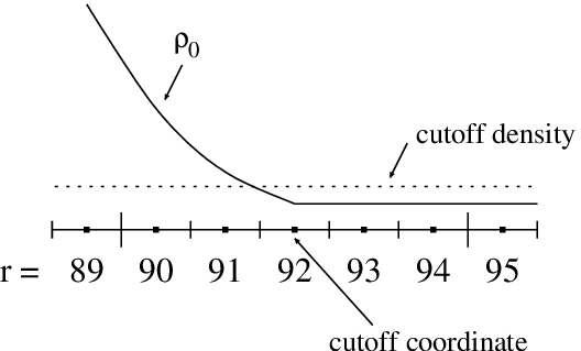
Fig. 16 Image of how the cutoff density and cutoff coordinates are related for single-level planar and all spherical problems.

Note that for single-level planar or any spherical problem, saying \(r\ge\) anelastic_cutoff_density_coord is analogous to saying \(\rho_0(r)\le\) anelastic_cutoff_density. Also, saying \(r<\) anelastic_cutoff_density_coord is analogous to saying \(\rho_0(r)>\) anelastic_cutoff_density. Ditto for base_cutoff_density and base_cutoff_density_coord.

Multilevel Planar

In this case, the base state exists as several one-dimensional arrays, each with different grid spacing. Refer to the figure below in the following examples. The guiding principle is to check whether \(\rho_0\) falls below \(\rho_{\rm cutoff}\) on the finest grid first. If not, check the next coarser level. Continue until you reach the base grid. Some examples are in order:

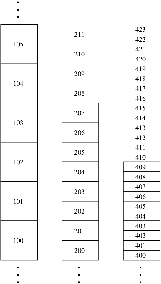
Fig. 17 Multilevel cutoff density example.

• Example 1: \(\rho_{0,104} > \rho_{\rm cutoff}\) and \(\rho_{0,105} < \rho_{\rm cutoff}\).

  cutoff_density_coord(1) = 105

  cutoff_density_coord(2) = 210

  cutoff_density_coord(3) = 420

  This is the simplest case in which the cutoff transition happens on the coarsest level. In this case, the cutoff coordinates at the finer levels are simply propagated from the coarsest level, even though they do not correspond to a valid region.
• Example 2: \(\rho_{0,403} > \rho_{\rm cutoff}\) and \(\rho_{0,404} < \rho_{\rm cutoff}\).

  cutoff_density_coord(1) = 101

  cutoff_density_coord(2) = 202

  cutoff_density_coord(3) = 404

  In this case, the cutoff transition happens where the finest grid is present. Happily, the transition occurs at a location where there is a common grid boundary between all three levels. Therefore, we simply propagate the cutoff density coordinate from the finest level downward.
• Example 3: \(\rho_{0,404} > \rho_{\rm cutoff}\) and \(\rho_{0,405} < \rho_{\rm cutoff}\).

  cutoff_density_coord(1) = 102

  cutoff_density_coord(2) = 203

  cutoff_density_coord(3) = 405

  In this case, the cutoff transition happens where the finest grid is present. However, the transition occurs at a location where there NOT is a common grid boundary between all three levels. We choose to define the cutoff transition at the coarser levels as being at the corresponding boundary that is at a larger radius than the location on the finest grid.

Note: if \(\rho_0\) does not fall below \(\rho_{\rm cutoff}\) at any level, we set the cutoff coordinate at the fine level to be first first cell above the domain and propagate the coordinate to the coarser levels.

When are the Cutoff Coordinates Updated?

At several points in the algorithm, we compute anelastic_cutoff_density_coord(:), base_cutoff_density_coord(:), and burning_cutoff_density_coord(:):

• After we call initialize in varden.

• After reading the base state from a checkpoint file when restarting.

• After regridding.

• After advancing \(\rho_0\) with advect_base_dens.

• After advancing \(\rho\) and setting \(\rho_0 = \overline{\rho}\).

• At the beginning of the second-half of the algorithm (Step 6), we reset the coordinates to the base-time values using \(\rho_0^n\).

Usage of Cutoff Densities

anelastic_cutoff_density

The anelastic_cutoff_density is the density below which we modify the constraint.

• In probin, anelastic_cutoff_density is set to \(-1\) by default. The user must supply a value in the inputs file or the code will abort.

• In make_div_coeff, for \(r \ge {\tt anelastic\_cutoff\_coord}\), we set \({\tt div\_coeff}(n,r) = {\tt div\_coeff}(n,r-1) * \rho_0(n,r)/\rho_0(n,r-1)\).

• in make_S, we set delta_gamma1_term and delta_gamma1 to zero for \(r \ge {\tt anelastic\_cutoff\_coord}\). This is only relevant if you are running with use_delta_gamma1_term = T.

• Some versions of sponge, use anelastic_cutoff_density in a problem dependent way.

base_cutoff_density

The base_cutoff_density is the lowest density that we model.

• In probin, base_cutoff_density is set to \(-1\) by default. The user must supply a value in the inputs file or the code will abort.

• In base_state, we compute a physical cutoff location, base_cutoff_density_loc, which is defined as the physical location of the first cell-center at the coarsest level for which \(\rho_0 \le {\tt base\_cutoff\_density}\). This is a trick used for making the data consistent for multiple level problems. When we are generating the initial background/base state, if we are above base_cutoff_density_loc, just use the values for \(\rho,T\), and \(p\) at base_cutoff_density_loc. When we check whether we are in HSE, we use base_cutoff_density_loc.

• In make_S_nodal, make_macrhs, and make_w0, we only add the volume discrepancy for \(r < {\tt base\_cutoff\_density\_coord}\) (in plane parallel) and if \(\rho_0^{\rm cart} > {\tt base\_cutoff\_density}\) (in spherical).

• In mkrhohforce for plane-parallel, for \(r \ge {\tt base\_cutoff\_density\_coord}\), we compute \(\nabla p_0\) with a difference stencil instead of simply setting it to \(\rho_0 g\).

• In update_scal, if \(\rho \le {\tt base\_cutoff\_density}\) and do_eos_h_above_cutoff, we call the EOS to compute \(h\).

• In update_scal, if \(\rho \le {\tt base\_cutoff\_density}/2\) we set it to \({\tt base\_cutoff\_density}/2\).

• In make_grav for spherical, we only add the enclosed mass if \(\rho_0 > {\tt base\_cutoff\_density}\).

• In enforce_HSE, we set \(p_0(r+1) = p_0(r)\) for \(r \ge {\tt base\_cutoff\_density\_coord}\).

• In make_psi for plane-parallel, we only compute \(\psi\) for \(r < {\tt base\_cutoff\_density\_coord}\).

burning_cutoff

The burning cutoff determines where we call the reaction network to get the nuclear energy generation rate and composition changes. For densities below the burning cutoff, we do not call the network.

• In probin, burning_cutoff_density is set to base_cutoff_density it no value is supplied.

• In react_state, we only call the burner if \(\rho >\) burning_cutoff_density.

buoyancy_cutoff_factor

The buoyancy_cutoff_factor is used to zero out the forcing terms to the velocity equation at low densities.

• In init_base_state we print out the value of the the density at which the buoyancy cutoff would take effect, buoyancy_cutoff_factor * base_cutoff_density.

• In mk_vel_force, we zero out rhopert, the perturbational density used in computing the buoyancy force, if \(\rho < \mathtt{buoyancy\_cutoff\_factor * base\_cutoff\_density}\).

• In mk_vel_force, for spherical problems, we zero out centrifugal_term, the centrifugal force for rotating stars, if \(\rho < \mathtt{buoyancy\_cutoff\_factor * base\_cutoff\_density}\).

• In make_explicit_thermal, if limit_conductivity = T, then for \(\rho < \mathtt{buoyancy\_cutoff\_factor}\)

  \(* \mathtt{base\_cutoff\_density}\), we zero out the thermal coefficients, effectively turning off thermal diffusion there.