Initial Models

Here we briefly describe the various routines for generating initial models for the main MAESTROeX problems and how the initial model is used to initialize both the base state and the full Cartesian state.

Note

When run, MAESTROeX outputs info that’s useful to check, including dr of base state and dr of the input file, which should be the same at the finest level; and Maximum HSE Error, which should be some small number.

Creating the Model Data from Raw Data

We have found that for the best performance, the MAESTROeX initialization procedure should be given model data with the same resolution as the base state resolution, \(\Delta r\).

• For planar problems, \(\Delta r = \Delta x\).

• For multilevel planar problems, we use \(\Delta r\) equal to \(\Delta x\) at the finest resolution.

• For spherical problems we set \(\Delta r = \Delta x/\mathtt{drdxfac}\).

We generate our initial model either analytically or from raw data, \(\rho^{\raw}, T^{\raw}, p^{\raw}\), and \(X^{\raw}\).

Here is the raw data file for each test problem:

(95)\[\begin{split}\begin{aligned} {\tt reacting\_bubble} & \rightarrow & \mathrm{none-it~ is~ generated~ analytically} \nonumber \nonumber \\ {\tt test\_convect} & \rightarrow & \mathrm{none-it~ is~ generated~ analytically} \nonumber \nonumber \\ {\tt wdconvect} & \rightarrow & {\tt model\_6.e8.raw} \nonumber \\ {\tt spherical\_heat} & \rightarrow & \mathrm{none-it~ is~ generated~ analytically} \nonumber \\\end{aligned}\end{split}\]

We use a fortran subroutine to interpolate the raw data, yielding the model data, \(\rho^{\model}, T^{\model}, p^{\model}\), and \(X^{\model}\). The fortran subroutine then uses an iterative procedure to modify the model data so that it is thermodynamically consistent with the MAESTROeX equation of state (EOS), and also satisfies our chosen hydrostatic equilibrium (HSE) discretization,

(96)\[\frac{p_r - p_{r-1}}{\Delta r} = \frac{\rho_r + \rho_{r-1}}{2}g_{r-\myhalf},\]

to a user defined tolerance. The shared initial_models git repo (https://github.com/AMReX-Astro/initial_models) has the routines used for creating initial models. Here are the names of the initial_models directories used for different problems:

problem name	initial_models routine
reacting_bubble	test2
test_convect	test2
wdconvect	none
spherical_heat	spherical

The model data is not generated at run-time—it must be generated in advance of running any MAESTROeX examples. The inputs file should point to the file containing the model data.

Creating the Initial Data from the Model Data

In base_state.f90, using the subroutine init_base_state (which is actually a terrible name since we are computing 1D initial data, which is not quite the same thing as the base satte), we set the initial data \(\rho^{\init}, T^{\init}, p^{\init}\) and \(X^{\init}\) equal to the model data. Then, we set \(p^{\init},h^{\init} = p,h(\rho^{\init},T^{\init},X^{\init})\) through the EOS. Note that we overwrite the existing value of \(p^{\init}\) but this should not change the value since we called \(p^{\model} = p^{\model}(\rho^{\model},T^{\model},X^{\model})\) at the end of the initial model generation routines in § 1.

For multilevel planar problems, we generate initial data at the non-finest levels by using linear interpolation from the two nearest model points (see the figure below). Note that the initial data is not in HSE nor is it thermodynamically consistent on non-finest cells. We will enforce these on the base state and full state later.

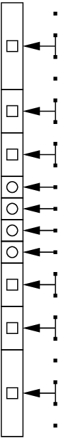
Fig. 11 Multilevel Initialization. The data from the initial model is represented by the dots on the right. The initial data at the finest level is represented by the circles. The initial data at non-finest levels is represented by the squares. We copy data from the dots directly into the circles. We use linear interpolation using the two nearest points to copy data from the dots to the squares.

We deal with the edge of the star by tracking the first coarse cell in which the density falls below base_cutoff_density. We note the radius of this cell center, and the values of \(\rho\), \(\rho h\), \(X_k\), \(p\), and \(T\) in this cells. Then, at every level, if current cell-center is above this radius, we set the state equal to this stored state. This ensures a consistent treatment of the edge of the star at all levels.

Creating the Base State and Full State

Given \(p^{\init}, \rho^{\init}, T^{\init},\) and \(X^{\init}\), this section describes how the base state (\(\rho_0\) and \(p_0\)) and full state (\(\rho, h, X\), and \(T\)) are computed. The base state is, general, not simply a direct copy of the initial model data, since we require that \(\rho_0 = \overline\rho\). Additionally, we require thebase state to be HSE according to Eq.96, and that the full state is thermodynamically consistent with \(p_0\). Overall we do:

1. Fill \(\rho^{\init}, h^{\init}, X^{\init}\), and \(T^{\init}\) onto a multifab to obtain the full state \(\rho, h, X\), and \(T\).

2. If perturb_model = T, a user-defined perturbation is added. This routine should make sure that the EOS is called so that there is some sense of thermodynamic consistency.

3. Set \(\rho_0 = \overline\rho\).

4. Compute \(p_0\) using enforce_HSE.

5. Compute \(T,h = T,h(\rho,p_0,X_k)\).

6. Set \((\rho h)_0 = \overline{(\rho h)}\).

7. Compute \(\overline{T}\). Note that we only use \(\overline{T}\) as a diagnostic and as a seed for EOS calls.

Now \(\rho_0 = \overline\rho\), the base state is in HSE, and the full state is thermodynamically consistent with \(p_0\).

Coarse-Fine enforce_HSE Discretization

When integrating the HSE discretization upward, we must use a different differencing procedure at coarse-fine interfaces. The figure below shows the transition from coarse (level \(l-1\)) to fine (level \(l\)), with the zone center indices noted.

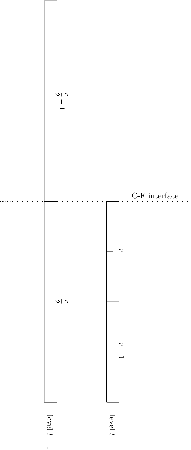
Fig. 12 A coarse-fine interface in the 1-d base state

To find the zone-centered pressure in the first fine zone, \(p_r^l\), from the zone-centered pressure in the coarse zone just below the coarse-fine interface, \(p_{r/2-1}^{l-1}\), we integrate in 2 steps. We allow for a spatially changing gravitational acceleration, for complete generality.

First we integrate up to the coarse-fine interface from the coarse-cell center as:

(97)\[\frac{p_{r-\myhalf}^l - p_{r/2-1}^{l-1}}{\Delta r^{l-1}/2} = \frac{\rho_{r-\myhalf}^l + \rho_{r/2-1}^{l-1}}{2} \, \frac{g_{r-\myhalf}^l + g_{r/2-1}^{l-1}}{2}\]

We can rewrite this as an expression for the pressure at the coarse-fine interface:

(98)\[p_{r-\myhalf}^l = p_{r/2-1}^{l-1} + \frac{\Delta r^{l-1}}{8} \left(\rho_{r-\myhalf}^l + \rho_{r/2-1}^{l-1}\right) \left(g_{r-\myhalf}^l + g_{r/2-1}^{l-1}\right).\]

Next we integrate up from the coarse-fine interface to the fine-cell center:

(99)\[\frac{p_r^l - p_{r-\myhalf}^l}{\Delta r^l/2} = \frac{\rho_r^l + \rho_{r-\myhalf}^l}{2} \, \frac{g_r^l + g_{r-\myhalf}^l}{2}\]

We can rewrite this as an expression for the pressure at the fine-cell center:

(100)\[p_r^l = p_{r-\myhalf}^l + \frac{\Delta r^l}{8} \left(\rho_r^l + \rho_{r-\myhalf}^l\right) \left(g_r^l + g_{r-\myhalf}^l\right).\]

Combining Eq.98 and Eq.100 gives

(101)\[\begin{split}\begin{align} p_r^l = p_{r/2-1}^{l-1} &+ \frac{\Delta r^{l-1}}{8} \left(\rho_{r-\myhalf}^l + \rho_{r/2-1}^{l-1}\right) \left( g_{r-\myhalf}^l + g_{r/2-1}^{l-1}\right) \nonumber \\ &+ \frac{\Delta r^l}{8} \left(\rho_r^l + \rho_{r-\myhalf}^l\right) \left( g_r^l + g_{r-\myhalf}^l\right).\end{align}\end{split}\]

We can simplify using

(102)\[\Delta r^{l-1} = 2\Delta r^l,\]

and by interpolating the cell-centered densities to the coarse-fine interface as:

(103)\[\rho_{r-\myhalf}^l = \frac{2}{3}\rho_r^l + \frac{1}{3}\rho_{r/2-1}^{l-1}.\]

Because we carry both the cell- and edge-centered gravitational accelerations, we do not need to interpolate \(g\) to the interface. Simplifying, we have

(104)\[\begin{split}\begin{align} p_r^l = p_{r/2-1}^{l-1} &+ \frac{\Delta r^l}{4}\left(\frac{2}{3}\rho_r^l + \frac{4}{3}\rho_{r/2-1}^{l-1} \right) \left( g_{r-\myhalf}^l + g_{r/2-1}^{l-1}\right) \nonumber \\ &+ \frac{\Delta r^l}{8}\left(\frac{5}{3}\rho_r^l + \frac{1}{3}\rho_{r/2-1}^{l-1}\right) \left( g_r^l + g_{r-\myhalf}^l\right) .\end{align}\end{split}\]

Finally, we note for constant \(g\), this simplifies to:

(105)\[p_r^l = p_{r/2-1}^{l-1} + \frac{3\Delta r^l g}{4}\left(\rho_{r/2-1}^{l-1} + \rho_r^l\right).\label{Coarse-Fine Stencil}\]

When integrating across a fine-coarse interface (see the figure below), the proceduce is similar.

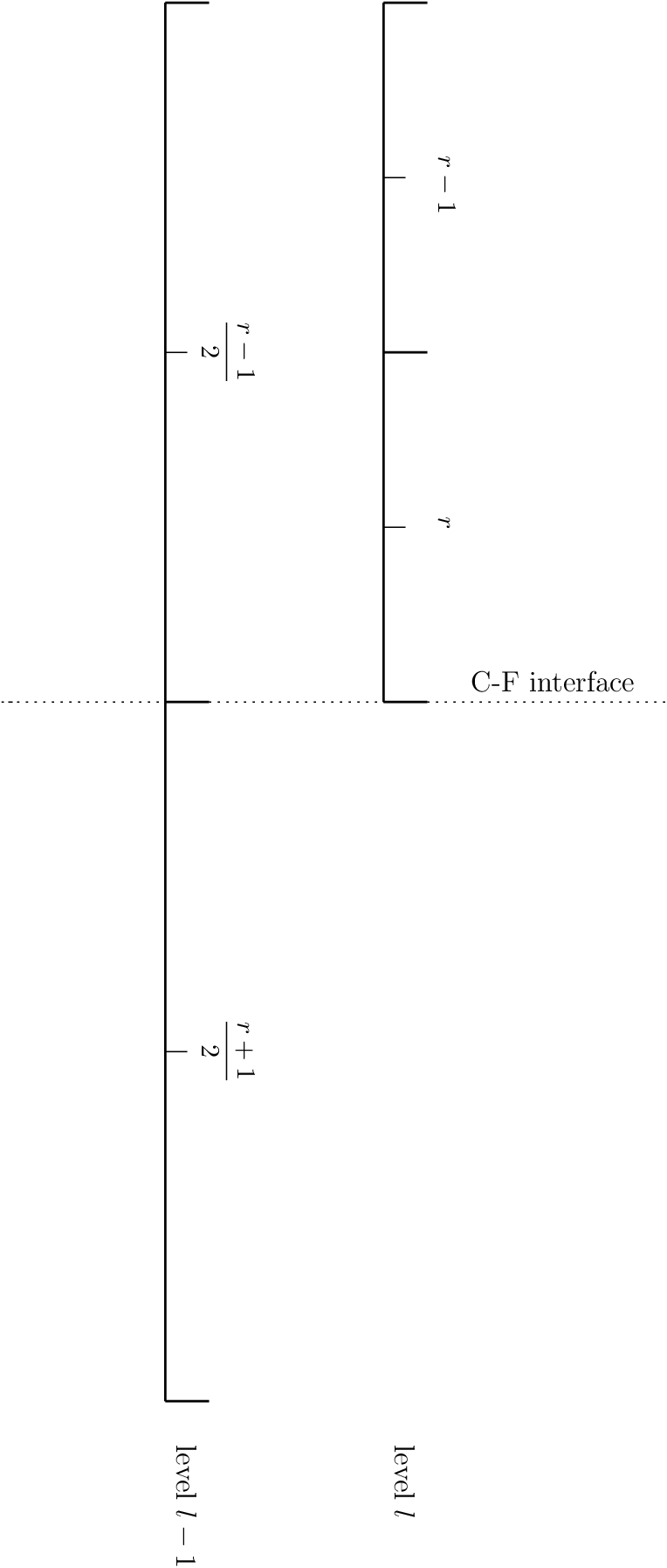
Fig. 13 A fine-coarse interface in the 1-d base state

The expression for general gravity becomes:

(106)\[\begin{split}\begin{align} p_{(r+1)/2}^{l-1} = p_{r}^l &+ \frac{\Delta r^l}{4}\left(\frac{2}{3}\rho_r^l + \frac{4}{3}\rho_{(r+1)/2}^{l-1} \right) \left( g_{(r+1)/2 -\myhalf}^{l-1} + g_{(r+1)/2}^{l-1}\right) \nonumber \\ &+ \frac{\Delta r^l}{8}\left(\frac{5}{3}\rho_r^l + \frac{1}{3}\rho_{(r+1)/2}^{l-1}\right) \left( g_r^l + g_{(r+1)/2 -\myhalf}^{l-1} \right) .\end{align}\end{split}\]

and for spatially-constant gravity, it simplifies to:

(107)\[p_{(r+1)/2}^{l-1} = p_{r}^l + \frac{3\Delta r^l g}{4}\left(\rho_{r}^l+\rho_{(r+1)/2}^{l-1}\right).\label{Fine-Coarse Stencil}\]