Unit Tests
In addition to the MAESTROeX science problems, which use the full capabilities of MAESTROeX, there are a number of unit tests that exercise only specific components of the MAESTROeX solvers. These tests have their own drivers (a custom varden.f90) that initialize only the data needed for the specific test and call specific MAESTROeX routines directly.
test_advect
This test initializes a Gaussian density field (no other scalar quantities are used) and a uniform velocity field in any one of the coordinate directions. The Gaussian profile is advected through the period domain exactly once and the error in the density profile (L2 norm) is computed. The driver for this problem does this for every dimension twice (once with a positive velocity and once with a negative velocity), and loops over all advection methods (ppm_type = 0,1,2 and bds_type = 1). After all coordinate directions are tested, the norms are compared to ensure that the error does not show any directional bias.
Note: the BDS advection method does not guarantee that the error be independent of the advection direction—small differences can arise. What’s happening here is that within each cell BDS is trying to define a tri-linear profile for rho subject to the constraints in the BDS paper ([NonakaMayAlmgrenBell11]) (constraints 1 and 2 on p. 2044 after eq. 3.4). We do not solve the L2 minimization problem exactly so we iterate up to 3 times using a simple heuristic algorithm designed to work toward the constraint. The iteration will give different results depending on orientation since we work through the corners in arbitrary order.
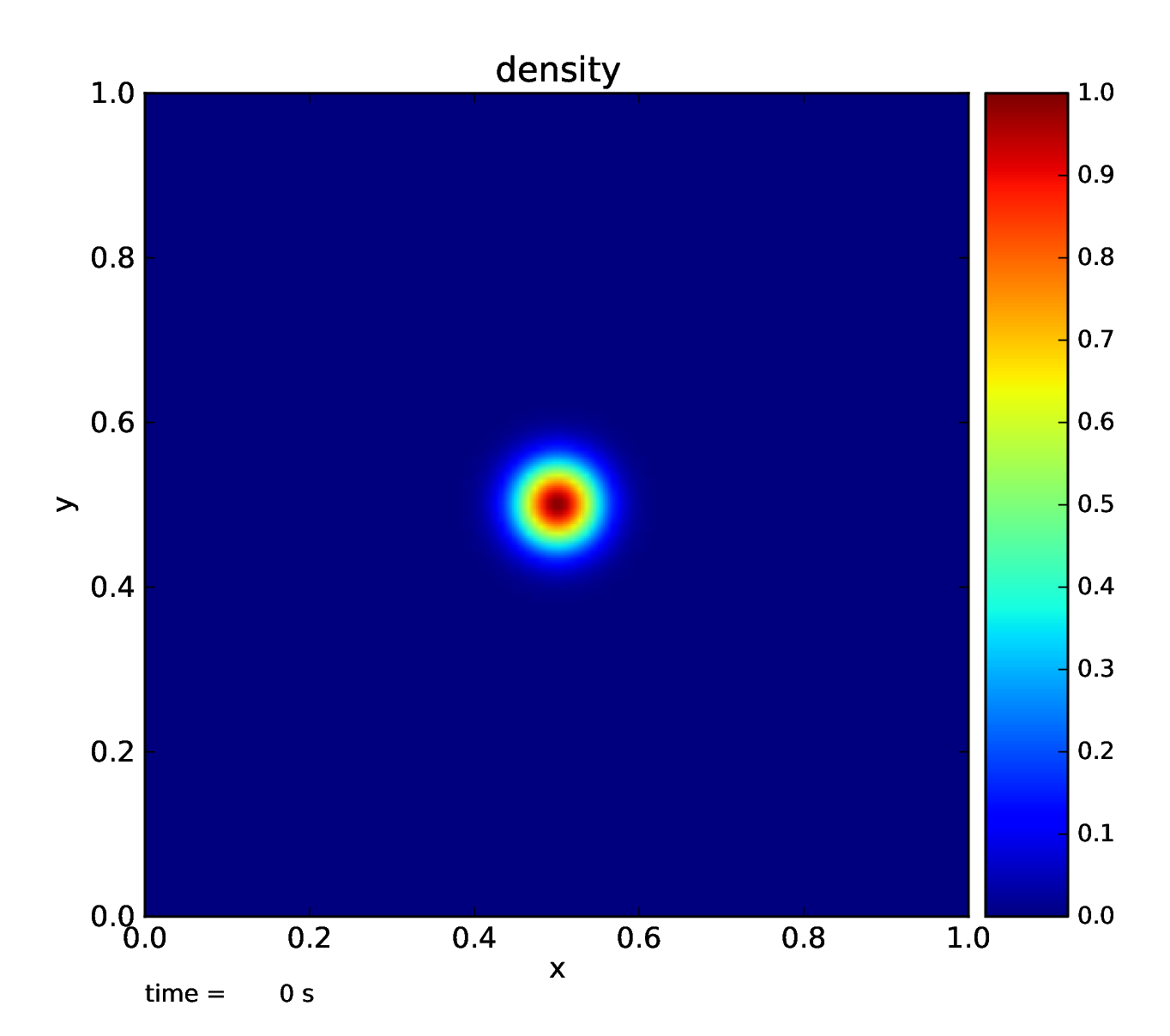
Fig. 4 Initial Gaussian density profile
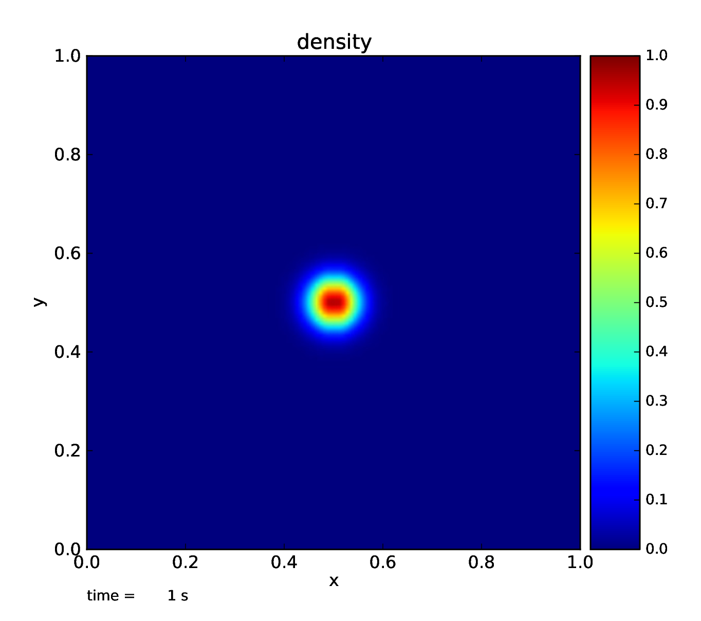
Fig. 5 density profile after advecting to the right for one period
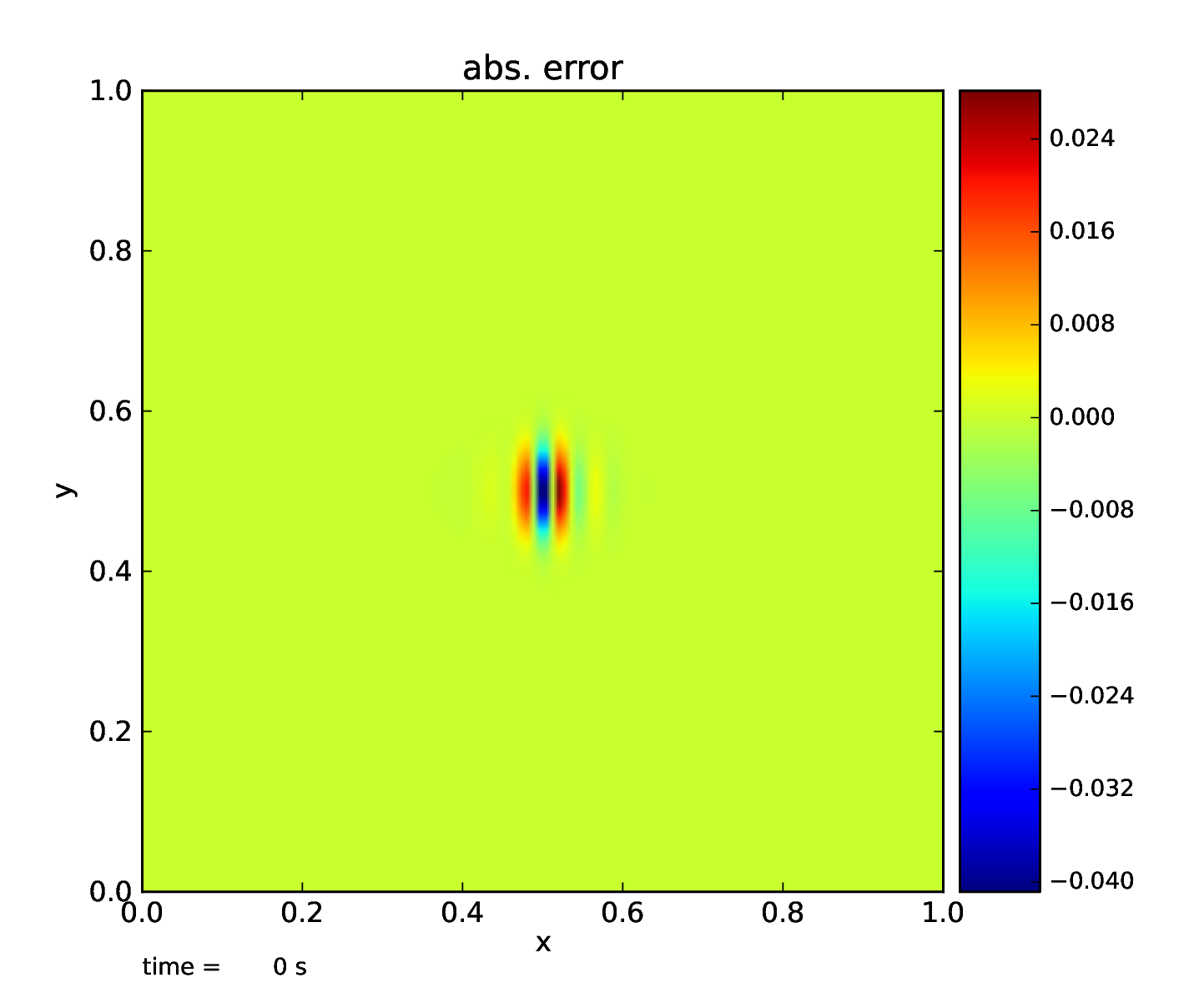
Fig. 6 absolute error between the final and initial density fields, showing the error in the advection scheme
test_average
This test initializes a 1D radial base state quantity with a Gaussian distribution, maps it into the 3D domain (assuming a spherical geometry) using the routines provided by the fill_3d_module module, and then calls average to put it back onto a 1D radial array. This way we test the accuracy of our procedure to map between the 1D radial and 3D Cartesian states. The output from this test was described in detail in [NonakaAlmgrenBell+10].
test_basestate
This test initializes the base state to contain a hydrostatic model and then evolves the state with heating to watch the hydrostatic adjustment of the atmosphere. In particular, the base state velocity, \(w_0\), is computed in response to the heating and this is used to advect the base state density and compute the new pressure, \(p_0\). An early version of this routine was used for the plane-parallel expansion test in [AlmgrenBellRendlemanZingale06b]. This version of the test was also shown for a spherical, self-gravitating star in [NonakaAlmgrenBell+10].
test_diffusion
This test initializes a Gaussian temperature profile and calls the thermal diffusion routines in MAESTROeX to evolve the state considering only diffusion. The driver estimates a timestep based on the explicit thermal diffusion timescale and loops over calls to the thermal diffusion solver. A Gaussian remains Gaussian when diffusing, so an explicit error can be computed by comparing to the analytic solution. This test is described in [MaloneNonakaAlmgren+11].
test_eos
This test sets up a 3-d cube with \(\rho\) varying on one axis, \(T\) on another, and the composition on the third. The EOS is then called in every zone, doing \((\rho, T) \rightarrow p, h, s, e\) and stores those quantities. Then it does each of the different EOS types to recover either \(T\) or \(\rho\) (depending on the type), and stores the new \(T\) (or \(\rho\)) and the relative error with the original value. A plotfile is stored holding the results and errors. This allows us to determine whether the EOS inversion routines are working right.
test_projection
This tests the projection routines in 2- and 3-d—either the hgprojection (project_type = 1) or the MAC projection (project_type = 2). A divergence-free velocity field is initialized and then “polluted” by adding the gradient of a scalar. The form of the scalar differs depending on the boundary conditions (wall and periodic are supported currently). Finally, the hgproject routine is called to recover the initial divergence-free field. The figures below show the initial field, polluted field, and result of the projection for the hgproject case.
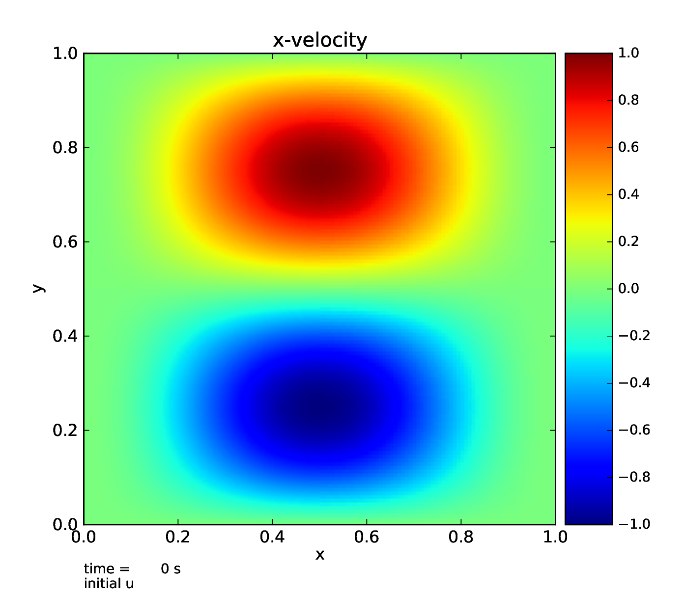
Fig. 7 Initial divergence free velocity field (x-component)
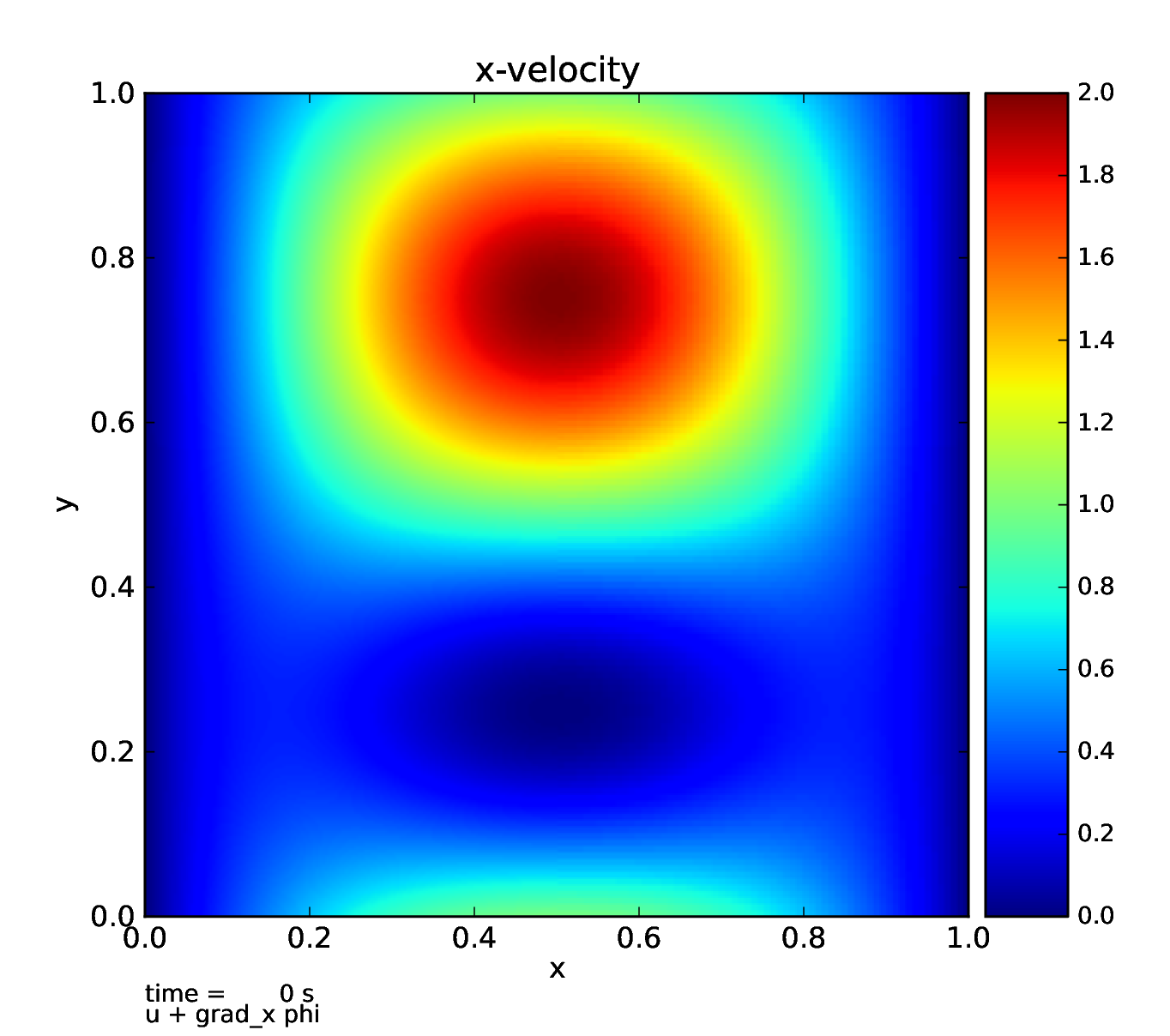
Fig. 8 Velocity field plus gradient of a scalar (x-component)
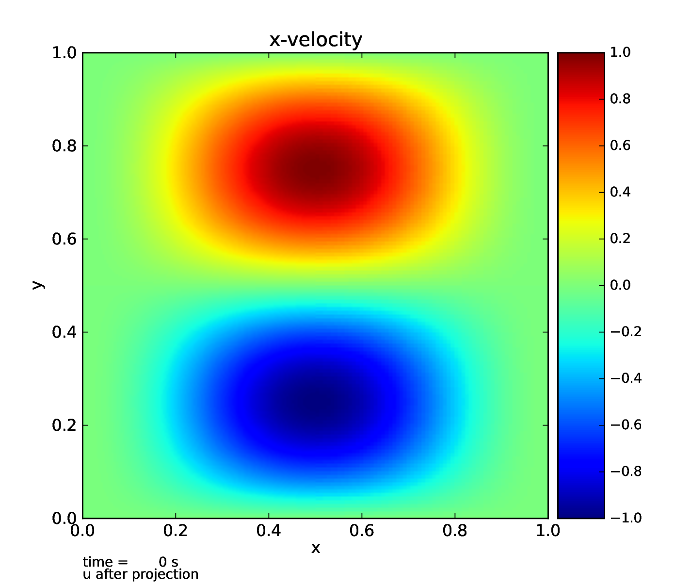
Fig. 9 Resulting velocity after projecting out the non-divergence free portion (x-component).
This is with slipwall boundary conditions on all sides, a 2-level grid with the left half refined and right half coarse, and the hgprojection tested.
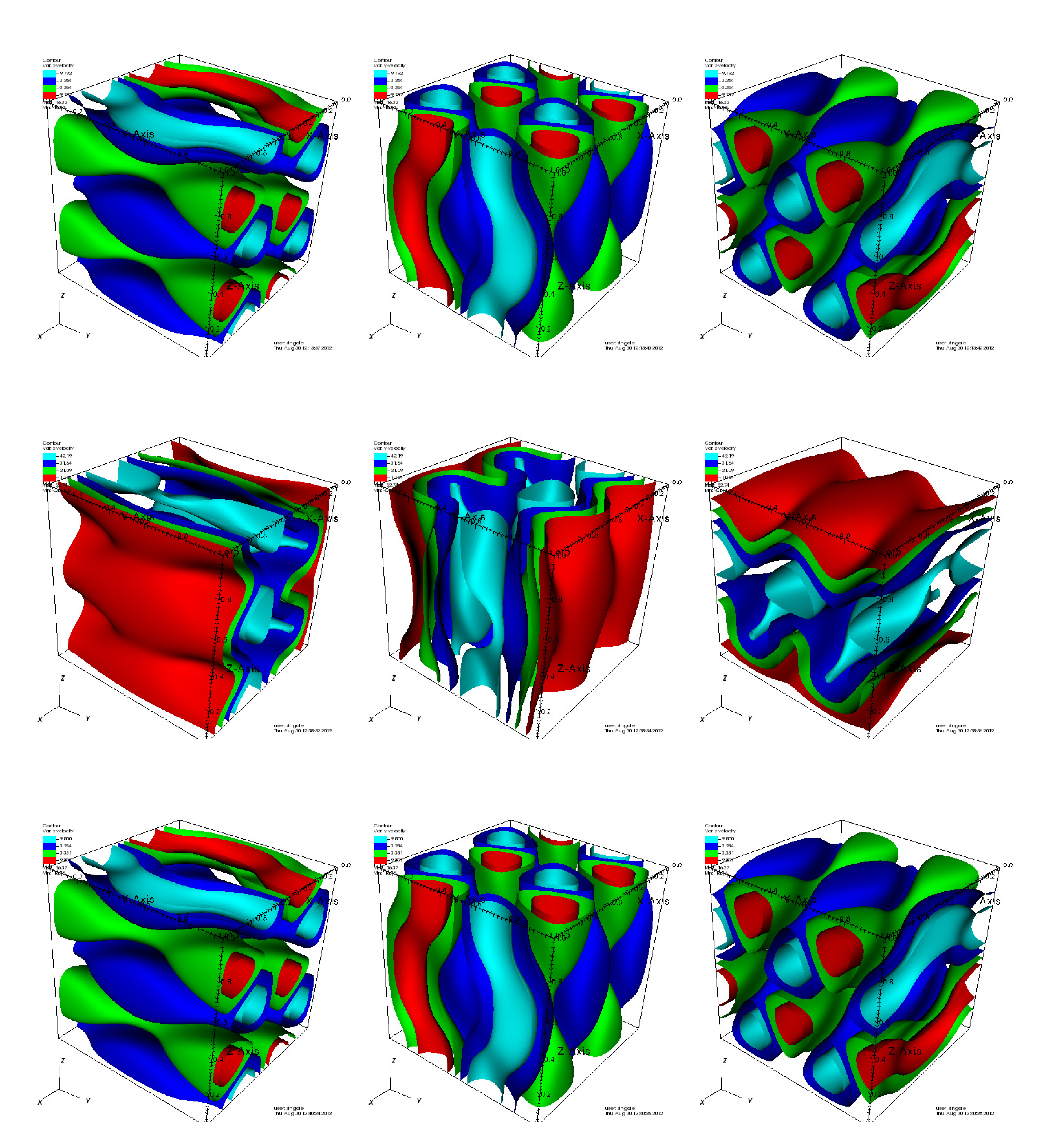
Fig. 10 Projection test in 3-d showing the x-velocity (left), y-velocity (middle), and z-velocity (right) initially (top row), after the gradient of a scalar is added (center row), and the resulting velocity after the projection. This is with slipwall boundary conditions on all sides, a 2-level grid with an octant refined, and the hgprojection.
test_react
This simply tests the reaction network by calling
the MAESTROeX react_state routine directly. The network is
selected in the GNUmakefile by setting the NETWORK_DIR
variable. A 3d cube is setup with density varying on one axis,
temperature varying on another, and the composition varying on the
third. The density and temperature ranges are set in the inputs
file. The composition is read in via an input file.
A good use of this test is to test whether a burner is threadsafe.
This is accomplished by compiling with OpenMP (setting OMP=t)
and the running with 1 thread and multiple threads (this can be done
by setting the environment variable OMP_NUM_THREADS to the
desired number of threads). Since each zone is independent of the
others, the results should be identical regardless of the number
of threads. This can be confirmed using the fcompare tool
in BoxLib/Tools/Postprocessing/F_Src/.