Multigrid

AMReX Multigrid Philosophy

Here we describe some of the general ideas behind the AMReX multigrid (MG).

We solve MG on an AMR hierarchy, which means in places we will encounter C-F interfaces. The AMReX MG will modify the stencil for the Laplacian at C-F interfaces to ensure the correct solution to the Poisson equation across these interfaces. There is no correction step needed in this case (this differs from [Ricker08]).

The MG solver always works with jumps of \(2\times\) between levels. In some codes (but not MAESTROeX) we can have jumps of \(4\times\) between levels. AMReX uses a mini_cycle in these cases, effectively inserting a multigrid level between the two AMR levels and doing a mini V-cycle.

The MG solvers are located in amrex/Src/LinearSolvers/F_MG/. There are two MG solvers, for cell-centered and nodal data. Generally, the routines specific to the cell-centered solver will have cc in their name, and those specific to the nodal solver will have nd in their name.

Support for \(\Delta x \ne \Delta y \ne \Delta z\)

Data Structures

mg_tower

The mg_tower is a special Fortran derived type that carries all the information required for a AMReX multigrid solve.

The following parameters are specified when building the mg_tower:

• smoother: the type of smoother to use. Choices are listed in mg_tower.f90. Common options are MG_SMOOTHER_GS_RB for red-black Gauss-Seidel and MG_SMOOTHER_JACOBI for Jacobi.

• nu1: The number of smoothings at each level on the way down the V-cycle.

• nu2: The number of smoothings at each level on the way up the V-cycle.

• nub: The number of smoothing before and after the bottom solver.

• gamma:

• cycle_type: The type of multigrid to do, V-cycles ( MG_VCycle), W-cycles (MG_WCycle), full multigrid ( MG_FCycle).

• omega:

• bottom_solver: the type of bottom solver to use. See the next section.

• bottom_max_iter: the maximum number of iterations for the bottom solver

• bottom_solver_eps: the tolerance used by the bottom solver. In MAESTROeX, this is set via mg_eps_module.

• max_iter: the maximum number of multigrid cycles.

• max_bottom_nlevel: additional coarsening if you use bottom_solver type 4 (see below)

• min_width: minimum size of grid at coarsest multigrid level

• rel_solver_eps: the relative tolerance of the solver (in MAESTROeX, this is set via mg_eps_module.

• abs_solver_eps: the absolute tolerance of the solver (in MAESTROeX, this is set via mg_eps_module.

• verbose: the verbosity of the multigrid solver. In MAESTROeX, this is set via the mg_verbose runtime parameter. Higher numbers give more verbosity.

• cg_verbose: the verbosity of the bottom solver. In MAESTROeX, this is set via the cg_verbose runtime parameter. Higher numbers give more verbosity.

In addition to these parameters, the mg_tower carries a number of multifabs that carry the solution and stencil for the multigrid solve.

• ss: The stencil itself—for each zone, this gives the coefficients of the terms in the Laplacian, with the convention that the ‘0’ term is located in the current cell and the other terms are the \(\pm 1\) off the current cell in each direction.

• cc: scratch space (?)

• ff: The source (righthand side) of the elliptic equation we are solving.

• dd: The residual/defect, \(f - L\phi\)

• uu: The solution variable (\(\phi\) when on the finest level)

• mm: For cell-centered, mm takes a direction and tells you whether we are at a Dirichlet or Neumann boundary, or if we are skewed in that direction.

  For nodal, mm simply tells us whether a point is Dirichlet or Neumann. There is no skew in nodal.

bndry_reg

There are two types of bndry_reg objects, each of which is a set of dim multifabs. The first, which is built with the bndry_reg_build call, is defined on all cells immediately outside of each grid. Each multifab within the bndry_reg contains all the fabs on both the low and high faces for a given direction. In the context of multigrid, we fill the bndry_reg with coarse data before interpolating the data to the correct locations to be used in the multigrid stencil. The second type of bndry_reg object is defined on the coarse cells immediately outside each fine grid, and is defined with the bndry_reg_rr_build call, is defined on all cells immediately outside. For this latter type, the option is available to include only cells not covered by a different fine grid, but this is left as an option because it requires additional calculations of box intersections.

In multigrid, we use the latter type of bndry_reg to calculate the residual at coarse cells adjacent to fine grids that is used as the right hand side in the relaxation step at the coarse level on the way down the V-cycle (or other). The first type of bndry_regis used to hold boundary conditions for the fine grids that are interpolated from the coarse grid solution; this is filled on the way back up the V-cycle.

To compute the residual in a coarse cell adjacent to a fine grid, we first compute the pure coarse residual, then subtract the contribution from the coarse face underlying the coarse-fine interface, and add the contribution of the fine faces at the coarse-fine interface. The bndry_reg holds the cell-centered contribution from the difference of these edge fluxes and is added to the coarse residual multifab.

Stencils

There are several different stencil types that we can use for the discretization. For cell-centered, these are:

• CC_CROSS_STENCIL: this is the standard cross-stencil—5 points in 2-d and 7 points in 3-d. For cell-centered MG, this is the default, and is usually the best choice.

• HO_CROSS_STENCIL: this is a cross-stencil that uses 9 points in 2-d and 11-points in 3-d. For instance, it will use \((i,j)\); \((i\pm1,j)\); \((i\pm2,j)\); \((i,j\pm1)\); \((i,j\pm2)\). This is higher-order accurate that CC_CROSS_STENCIL.

• HO_DENSE_STENCIL: this is a dense-stencil—it uses all the points (including corners) in \((i\pm1,j\pm1)\), resulting in a 9-point stencil in 2-d and 27-point stencil in 3-d.

For the nodal solver, the choices are:

• ND_CROSS_STENCIL: this is the standard cross-stencil.

• ND_DENSE_STENCIL: this is a dense stencil, using all the points in \((i\pm1,j\pm1)\). The derivation of this stencil is based on finite-element ideas, defining basis functions on the nodes. This is developed in 2-d in [ABS96].

• ND_VATER_STENCIL: this is an alternate dense stencil derived using a similar finite-element idea as above, but a different control volume.

For the cell-centered solve, the coefficients for the stencil are computed once, at the beginning of the solve. For the nodal solver, the coefficients are hard-coded into the smoothers.

Smoothers

The following smoothers are available (but not necessarily for both the cell-centered and nodal solvers):

• MG_SMOOTHER_GS_RB: a red-black Gauss-Seidel smoother

• MG_SMOOTHER_JACOBI: a Jacobi smoother (not implemented for the dense nodal stencil)

• MG_SMOOTHER_MINION_CROSS

• MG_SMOOTHER_MINION_FULL

• MG_SMOOTHER_EFF_RB

Cycling

The default cycling is a V-cycle, but W-cycles and full multigrid are supported as well.

Bottom Solvers

The multigrid cycling coarsens the grids as part of the solve. When the coarsest grid is reached, the individual boxes that comprise that level are coarsened as much as then can, down to \(2^3\) zones. Depending on the distribution of sizes of the grids, it may not be possible for everything to reach this minimum size. At this point, the bottom solver is invoked. Most of these will solve the linear system on this collection of grids directly. There is one special bottom solver that will define a new box encompassing all of the coarsened grids and then put the data on fewer boxes and processors and further coarsen the problem, again until we get as close to \(2^3\) as possible. At that point, one of the other bottom solvers will be called upon to solve the problem.

There are several bottom solvers available in AMReX. For MAESTROeX. These are set through the mg_bottom_solver (MAC/cell-centered) and hg_bottom_solver (nodal) runtime parameters. The allowed values are:

• mg_bottom_solver / hg_bottom_solver = 0: smoothing only.

• mg_bottom_solver / hg_bottom_solver = 1: biconjugate gradient stabilized—this is the default.

• mg_bottom_solver / hg_bottom_solver = 2: conjugate gradient method

• mg_bottom_solver / hg_bottom_solver = 4: a special bottom solver that extends the range of the multigrid coarsening by aggregating coarse grids on the original mesh together and further coarsening.

You should use the special bottom solver (4) whenever possible, even if it means changing your gridding strategy (as discussed below) to make it more efficient.

Special Bottom Solver

The special solver takes the data from the coarsest level of the original multigrid V-cycle and copies it onto a new grid structure with the same number of total cells in each direction, but with a fewer number of larger grids. A new V-cycle begins from this point, so we are essentially coarsening this “new” problem. Now, the coarsest level of the multigrid V-cycle in the “new” problem has fewer cells and fewer grids as compared to the original coarsest level.

To enable this solver, set hg_bottom_solver = 4 (for the nodal projections) and/or mg_bottom_solver = 4 (for the cell-centered projections) in your inputs file.

To understand how this bottom solver works, the first thing you need to know is what the grid structure of the coarsest level of your multigrid V-cycle looks like. Next, figure out the size of the box you would need if you wanted it to fit all the data on the coarsest level. Finally, figure out what the largest integer \(n\) is so that you can evenly divide the length of this box by \(2^n\) in every coordinate direction. If \(n < 2\), the program will abort since the grid structure is not suitable for this bottom solver.

The code will set up a “new” problem, using the data at the coarsest level of the original problem as the initial data. The grid structure for this new problem has the same number of cells as the coarsest level of the original problem, but the data is copied onto a grid structure where each grid has \(2^n\) cells on each side. The new V-cycle continues down to the new coarsest level, in which each grid has 2 cells on each side. If you wish to impose a limit on the maximum value that \(n\) can have, you can do so by setting max_mg_bottom_nlevs equal to that value.

Some grid examples help make this clear:

• Example 1: A 3D problem with \(384^3\) cells divided into \(32^3\) grids, i.e., there is a \(12\times 12\times 12\) block of \(32^3\) grids. The coarsest level of the multigrid V-cycle contains \(12\times 12\times 12\) grids that have \(2^3\) cells, so the entire problem domain has \(24^3\) cells. We see that \(n=3\), and create a new problem domain with a \(3\times 3\times 3\) block of \(8^3\) grids. The coarsest level of the multigrid V-cycle for the “new” problem will be a \(3\times 3\times 3\) block of \(2^3\) grids.

• Example 2: A 2D problem with \(96\times 384\) cells divided into \(48^2\) grids, i.e., there is a \(2\times 8\) block of \(48^2\) grids. The coarsest level of the multigrid V-cycle contains \(2\times 8\) grids that have \(3^2\) cells, so the entire problem domain has \(6\times 24\) cells. We see that \(n=0\), so the program aborts since this grid structure is not appropriate for the fancy bottom solver.

Flowchart

MAESTROeX multigrid solves always involve the full AMR hierarchy.

Cell-Centered MG

The flowchart below shows the structure of a cell-centered multigrid solve using pure V-cycles.

• stencil_fill_cc_all_mglevels / stencil_fill_cc: Compute all of the stencil coefficients for the Laplacian operator at all cells. At the C-F interfaces, the stencil coefficients are modified to know this.

• ml_cc: The main driver for the cell-centered multigrid. Among other things, this computes the norm that will be used for convergence testing.

• mg_tower_v_cycle (recursive):

  • recursively descend V-cycle

    • : Smooth the problem at the current MG level using the desired smoother.

    • compute_defect: Construct \(f - L\phi\).

    • : Restrict the defect to the coarser level by conservative averaging.

  • mg_tower_bottom_solve: Solve the coarsened problem using the chosen bottom solver.

  • ascend V-cycle

    • : Take the solution at level \(n-1\) and use it to correct the solution at level \(n\) by representing the data on the finer grid. This uses linear reconstruction for jumps by \(2\times\) and piecewise-constant otherwise.

    • :

• compute_defect: This is called multiple times, checking for convergence at each level.

Nodal MG

The flowchart below shows the structure of a cell-centered multigrid solve using pure V-cycles.

• stencil_fill_cc_all_mglevels / stencil_fill_cc: For the nodal solver, this applies the weights to the coefficients.

• ml_nd: The main driver for the nodal multigrid.

• mg_tower_v_cycle (recursive):

  • recursively descend V-cycle

    • : Smooth the problem at the current MG level using the desired smoother.

    • compute_defect: Construct \(f - L\phi\).

    • : Restrict the defect to the coarser level by simply taking the fine value that lies at the same place as the coarse data.

  • mg_tower_bottom_solve: Solve the coarsened problem using the chosen bottom solver.

  • ascend V-cycle

    • : For nodal data, the fine grid will have some points at exactly the same place as the coarse data—these are simply copied to the fine grid. The remain data is interpolated.

    • :

• compute_defect: This is called multiple times, checking for convergence at each level.

MAESTROeX’s Multigrid Use

MAESTROeX uses multigrid to enforce the velocity constraint through projections at the half-time (the MAC projection) and end of the time step (the HG projection). Two multigrid solvers are provided by AMReX—one for cell-centered data and one for node-centered (nodal) data. Both of these are used in MAESTROeX.

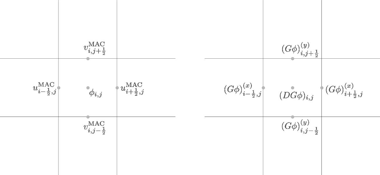
The MAC projection operates on the advective velocities predicted at the cell-interfaces at the half-time. The edge-centered velocities are shown in fig:mg:MAC. If we consider purely incompressible flow, the projection appears as:

(288)\[D G \phi = D U\]

where \(D\) is the divergence operator and \(G\) is the gradient operator. In this discretization, \(\phi\) is cell-centered (see fig:mg:MAC. The remaining quantities are discretized as:

• \(DU\) is cell-centered,

  (289)\[(DU)_{i,j} = \frac{u_{i+1/2,j} - u_{i-1/2,j}}{\Delta x} + \frac{v_{i,j+1/2} - v_{i,j-1/2}}{\Delta y}\]

• \(G\phi\) is edge-centered, on the MAC grid, as shown in fig:mg:MAC.

• \(DG\phi\) is cell-centered, also shown in fig:mg:MAC, computed from \(G\phi\) using the same differencing as \(DU\).

The HG projection projects the cell-centered velocities at the end of the timestep. Here, \(\phi\) is node-centered. fig:mg:HG shows the locations of the various quantities involved in the HG projection. Again considering simple incompressible flow, we now solve:

(290)\[L \phi = D U\]

where \(L\) is a discretization of the Laplacian operator. In this sense, the HG projection is an approximate projection, that is, \(L \neq DG\) (in discretized form). The various operations have the following centerings:

• \(DU\) is node-centered. This is computed as:

  (291)\[(DU)_{i-1/2,j-1/2} = \frac{\frac{1}{2} (u_{i,j} + u_{i,j-1}) - \frac{1}{2} (u_{i-1,j} + u_{i-1,j-1})}{\Delta x} + \frac{\frac{1}{2} (v_{i,j} + v_{i-1,j}) - \frac{1}{2} (v_{i,j-1} + v_{i-1,j-1})}{\Delta y}\]

• \(G\phi\) is cell-centered, as shown in fig:mg:HG.

• \(L\phi\) is node-centered. This is a direct discretization of the Laplacian operator. By default, MAESTROeX uses a dense stencil (9-points in 2-d, 27-points in 3-d). Alternately, a cross stencil can be used (by setting hg_dense_stencil = F). This uses 5-points in 2-d, 7-points in 3-d.

  

Convergence Criteria

All MAESTROeX multigrid solves consist of pure V-cycles.

Multigrid Solver Tolerances

Beginning at the start of execution, there are several places where either cell-centered multigrid or node-centered multigrid solves are performed. The outline below lists the solves one encounters, in order, from the start of execution. The values of the tolerances lists here are defined in the mg_eps module. To set problem-specific values of these tolerances, place a local copy of mg_eps.f90 in your problem directory.

In the initialization, multigrid comes in during the initial projection and the “divu” iterations.

• initial projection (initial_proj called from varden)

  The initial projection creates a first approximation to the velocity field by forcing the initial velocity field set by initveldata to satisfy the elliptic constraint equation. Since the initial velocity may be zero, there is no guarantee that a well-defined timestep can be computed at this point, so the source term, \(S\), used here only involves thermal diffusion and any external heating term, \(\Hext\)—no reactions are included (see paper III, §3.3).

  The initial projection can be disabled with the do_initial_projection runtime parameter.

  The tolerances, eps_init_proj_cart and eps_init_proj_sph (for Cartesian and spherical respectively) are set in mg_eps.f90 and have the default values of:

  Cartesian:	eps_init_proj_cart	= \(10^{-12}\)
  spherical:	eps_init_proj_sph	= \(10^{-10}\)

• “divu” iterations (divu_iter called from varden)

  The “divu” iterations projects the velocity field from the initial projection to satisfy the full constraint (including reactions). This is an iterative process since the reactions depend on the timestep and the timestep depends on the velocity field (see paper III, §3.3). The number of iterations to take is set through the init_divu_iter runtime parameter.

  The overall tolerance, \(\epsilon_\mathrm{divu}\) depends on the iteration, \(i\). We start with a loose tolerance and progressively get tighter. The tolerances (set in divu_iter) are, for Cartesian:

  (292)\[\begin{split}\epsilon_\mathrm{divu} = \left \{ \begin{array}{lll} \min\, \{& \!\!\!\mathtt{eps\_divu\_cart} \cdot \mathtt{divu\_iter\_factor}^2 \cdot \mathtt {divu\_level\_factor}^{(\mathtt{nlevs}-1)}, \\ & \!\!\!\mathtt{eps\_divu\_cart} \cdot \mathtt{divu\_iter\_factor}^2 \cdot \mathtt{divu\_level\_factor}^2 \, \} & \quad \mathrm{for}~ i \le \mathtt{init\_divu\_iter} - 2 \\[2mm] \min\, \{& \!\!\!\mathtt{eps\_divu\_cart} \cdot \mathtt{divu\_iter\_factor} \cdot \mathtt{divu\_level\_factor}^{(\mathtt{nlevs}-1)}, \\ & \!\!\!\mathtt{eps\_divu\_cart} \cdot \mathtt{divu\_iter\_factor} \cdot \mathtt{divu\_level\_factor}^2 \, \} & \quad \mathrm{for}~ i = \mathtt{init\_divu\_iter} - 1 \\[2mm] \min\, \{& \!\!\!\mathtt{eps\_divu\_cart} \cdot \mathtt{divu\_level\_factor}^{(\mathtt{nlevs}-1)}, \\ & \!\!\!\mathtt{eps\_divu\_cart} \cdot \mathtt{divu\_level\_factor}^2 \, \} & \quad \mathrm{for}~ i = \mathtt{init\_divu\_iter} \\ \end{array} \right .\end{split}\]

  and for spherical:

  (293)\[\begin{split}\epsilon_\mathrm{divu} = \left \{ \begin{array}{ll} \mathtt{eps\_divu\_sph} \cdot \mathtt{divu\_iter\_factor}^2 & \quad \mathrm{for}~ i \le \mathtt{init\_divu\_iter} - 2 \, \\[2mm] \mathtt{eps\_divu\_sph} \cdot \mathtt{divu\_iter\_factor} & \quad \mathrm{for}~ i = \mathtt{init\_divu\_iter} - 1 \, \\[2mm] \mathtt{eps\_divu\_sph} & \quad \mathrm{for}~ i = \mathtt{init\_divu\_iter} \, )\\ \end{array} \right .\end{split}\]

  The various parameters are set in mg_eps.f90 and have the default values of:

  eps_divu_cart	= \(10^{-12}\)
  eps_divu_sph	= \(10^{-10}\)
  divu_iter_factor	= 100
  divu_level_factor	= 10

In the main algorithm, mulitgrid solves come in during the two MAC projections, two (optional) thermal diffusion solves, and the final velocity projection.

• MAC projection

  The MAC projection forces the edge-centered, half-time advective velocities to obey the elliptic constraint. This is done both in the predictor and corrector portions of the main algorithm.

  There are two tolerances here. The norm of the residual is required to be reduced by a relative tolerance of

  (294)\[\epsilon = \min \{ \mathtt{eps\_mac\_max}, \mathtt{eps\_mac} \cdot \mathtt{mac\_level\_factor}^{(\mathtt{nlevs}-1)} \} .\]

  A separate tolerance is used for the bottom solver, \(\epsilon_\mathrm{bottom} = \mathtt{eps\_mac\_bottom}\). These parameters are set in mg_eps.f90 and have the default values:

  eps_mac	= \(10^{-10}\)
  eps_mac_max	= \(10^{-8}\)
  mac_level_factor	= 10
  eps_mac_bottom	= \(10^{-3}\)

• thermal diffusion

  This uses the same mac_multigrid routine as the MAC projection, so it uses the same tolerances. The only difference is that the absolute tolerance is based on the norm of \(h\) now, instead of \(U^\mathrm{ADV}\).

• velocity projection

  The final velocity projection uses a tolerance of :math:`epsilon = min {

  mathtt{eps_hg_max}, mathtt{eps_hg} cdot mathtt{hg_level_factor}^{(mathtt{nlevs} - 1)} }`. This tolerance

  is set in hgproject using the parameter values specified in mg_eps.f90. A separate tolerance is used for the bottom solver, \(\epsilon_\mathrm{bottom} = \mathtt{eps\_hg\_bottom}\).

  The default parameter values are:

  eps_hg	= \(10^{-12}\)
  eps_hg_max	= \(10^{-10}\)
  hg_level_factor	= 10
  eps_hg_bottom	= \(10^{-4}\)

General Remarks

If MAESTRO has trouble converging in the multigrid solves, try setting the verbosity mg_verbose or cg_verbose to higher values to get more information about the solve.