Rotation in MAESTROeX
Rotation
To handle rotation in MAESTROeX we move to the co-rotating reference frame. Time derivatives of a vector in the inertial frame are related to those in the co-rotating frame by
where i(rot) refers to the inertial(co-rotating) frame and \(\Omegab\) is the angular velocity vector. Using Eq.295 and assuming \(\Omegab\) is constant, we have
Plugging this into the momentum equation and making use of the continuity equation we have a momentum equation in the co-rotating frame:
The Coriolis and Centrifugal terms are force terms that will be added to right hand side of the equations in mk_vel_force. Note that the Centrifugal term can be rewritten as a gradient of a potential and absorbed into either the pressure or gravitational term to create an effective pressure or effective gravitational potential. Furthermore, because it can be written as a gradient, this term would drop out completely in the projection if we were doing incompressible flow. In what follows we will include the Centrifugal term explicitly.
Using Spherical Geometry
In spherical geometry implementing rotation is straightforward as we don’t have to worry about special boundary conditions. We assume a geometry as shown in Fig. 27 where the primed coordinate system is the simulation domain coordinate system, the unprimed system is the primed system translated by the vector \(\rb_\text{c}\) and is added here for clarity. The \(\rb_\text{c}\) vector is given by center in the geometry module. In spherical, the only runtime parameter of importance is rotational_frequency in units of Hz. This specifies the angular velocity vector which is assumed to be along the k direction:
The direction of \(\rb\) is given as the normal vector which is passed into mk_vel_force; in particular
The magnitude of \(\rb\) is calculated based on the current zone’s location with respect to the center. Using this notation we can write the Centrifugal term as
The Coriolis term is a straightforward cross-product:
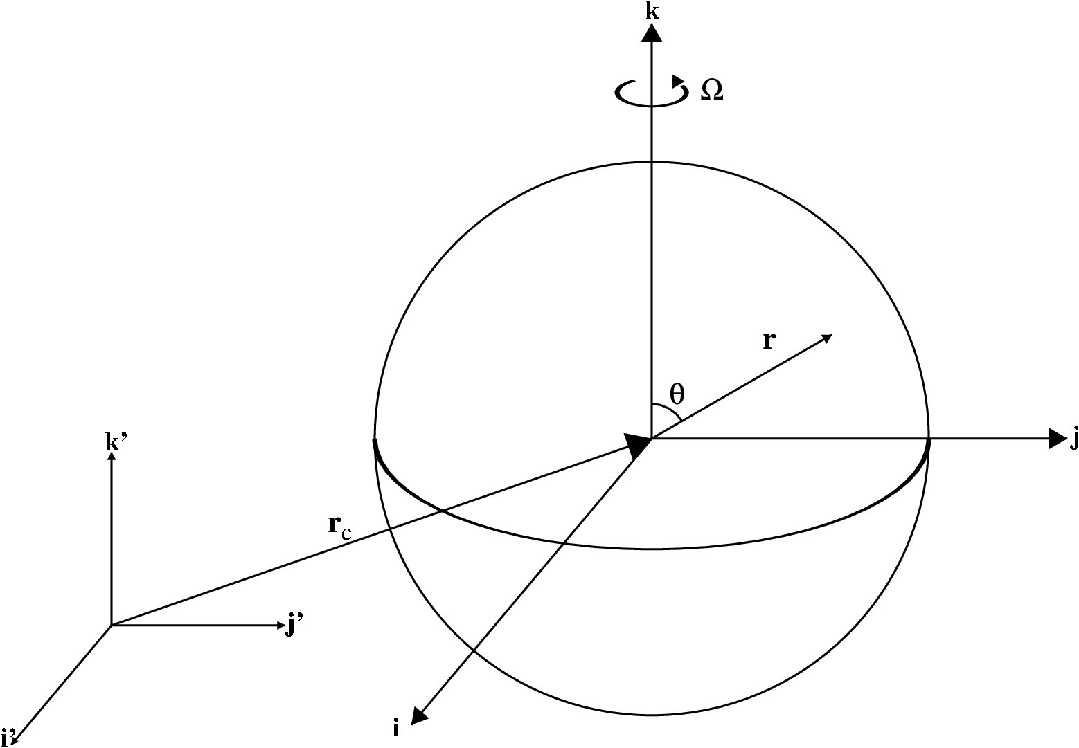
Fig. 27 Geometry of rotation when spherical_in \(=1\). We assume the star to be rotating about the \(z\) axis with rotational frequency \(\Omega\).