Interface State Details

Predicting interface states

The MAESTROeX hyperbolic equations come in two forms: advective and conservative. The procedure for predicting interface states differs slightly depending on which form we are dealing with.

Advective form

Most of the time, we are dealing with equations in advective form. Here, a scalar, \(\phi\), obeys:

(134)\[\frac{\partial \phi}{\partial t} = -\Ub \cdot \nabla \phi + f\]

where \(f\) is the force. This is the form that the perturbation equations take, as well as the equation for \(X_k\) itself.

A piecewise linear prediction of \(\phi\) to the interface would appear as:

(135)\[\begin{split}\begin{aligned} \phi_{i+1/2,j}^{n+1/2} &=& \phi_{i,j}^n + \left . \frac{\Delta x}{2} \frac{\partial \phi}{\partial x} \right |_{i,j} + \left . \frac{\Delta t}{2} \frac{\partial \phi}{\partial t} \right |_{i,j} \\ &=& \phi_{i,j}^n + \left . \frac{\Delta x}{2} \frac{\partial \phi}{\partial x} \right |_{i,j} + \frac{\Delta t}{2} \left ( -u \frac{\partial \phi}{\partial x} -v \frac{\partial \phi}{\partial y} + f \right ) \\ &=& \phi_{i,j}^n + \frac{\Delta x}{2} \left ( 1 - \frac{\Delta t}{\Delta x} u \right ) \frac{\partial \phi}{\partial x} \underbrace{- \frac{\Delta t}{2} v \frac{\partial \phi}{\partial y}}_{\text{``transverse~term''}} + \frac{\Delta t}{2} f\end{aligned}\end{split}\]

(see the Godunov notes section for more details). Here, the “transverse term” is accounted for in make_edge_scal. Any additional forces should be added to \(f\). For the perturbation form of equations, we add additional advection-like terms to \(f\) by calling modify_scal_force. This will be noted below.

Conservative form

A conservative equation takes the form:

(136)\[\frac{\partial \phi}{\partial t} = -\nabla \cdot ( \phi \Ub) + f\]

Now a piecewise linear prediction of \(\phi\) to the interface is

(137)\[\begin{split}\begin{aligned} \phi_{i+1/2,j}^{n+1/2} &=& \phi_{i,j}^n + \left . \frac{\Delta x}{2} \frac{\partial \phi}{\partial x} \right |_{i,j} + \left . \frac{\Delta t}{2} \frac{\partial \phi}{\partial t} \right |_{i,j} \\ &=& \phi_{i,j}^n + \left . \frac{\Delta x}{2} \frac{\partial \phi}{\partial x} \right |_{i,j} + \frac{\Delta t}{2} \left ( -\frac{\partial (\phi u)}{\partial x} -\frac{\partial (\phi v)}{\partial y} + f \right ) \\ &=& \phi_{i,j}^n + \frac{\Delta x}{2} \left ( 1 - \frac{\Delta t}{\Delta x} u \right ) \frac{\partial \phi}{\partial x} \underbrace{- \frac{\Delta t}{2} \phi \frac{\partial u}{\partial x} }_{\text{``non-advective~term''}} \underbrace{- \frac{\Delta t}{2} \frac{\partial (\phi v)}{\partial y}}_{\text{``transverse~term''}} + \frac{\Delta t}{2} f\end{aligned}\end{split}\]

Here the “transverse term” is now in conservative form, and an additional term, the non-advective portion of the \(x\)-flux (for the \(x\)-prediction) appears. Both of the underbraced terms are accounted for in make_edge_scal automatically when we call it with is_conservative = .true..

Density Evolution

Basic equations

The full density evolution equation is

(138)\[\begin{split}\begin{aligned} \frac{\partial\rho}{\partial t} &=& -\nabla\cdot(\rho\Ub) \nonumber \\ &=& -\Ub\cdot\nabla\rho - \rho\nabla\cdot\Ub \, . \end{aligned}\end{split}\]

The species are evolved according to

(139)\[\begin{split}\begin{aligned} \frac{\partial(\rho X_k)}{\partial t} &=& -\nabla\cdot(\rho\Ub X_k) + \rho \omegadot_k \nonumber \\ &=& -\Ub\cdot\nabla(\rho X_k) - \rho X_k \nabla\cdot\Ub + \rho \omegadot_k \, . \end{aligned}\end{split}\]

In practice, only the species evolution equation is evolved, and the total density is set as

(140)\[\rho = \sum_k (\rho X_k)\]

To advance \((\rho X_k)\) to the next timestep, we need to predict a time-centered, interface state. Algebraically, there are multiple paths to get this interface state—we can predict \((\rho X)\) to the edges as a single quantity, or predict \(\rho\) and \(X\) separately (either in full or perturbation form). In the notes below, we use the subscript ‘edge’ to indicate what quantity was predicted to the edges. In MAESTROeX, the different methods of computing \((\rho X)\) on edges are controlled by the species_pred_type parameter. The quantities predicted to edges and the resulting edge state are shown in the Table 4.

Table 4 Summary of species edge state construction

species_pred_type	quantities predicted in make_edge_scal	\((\rho X_k)\) edge state
1 / predict_rhoprime_and_X	\(\rho'_\mathrm{edge}\), \((X_k)_\mathrm{edge}\)	\(\left(\rho_0^{n+\myhalf,{\rm avg}} + \rho'_\mathrm{edge} \right)(X_k)_\mathrm{edge}\)
2 / predict_rhoX	\(\sum(\rho X_k)_\mathrm{edge}\), \((\rho X_k)_\mathrm{edge}\)	\((\rho X_k)_\mathrm{edge}\)
3 / predict_rho_and_X	\(\rho_\mathrm{edge}\), \((X_k)_\mathrm{edge}\)	\(\rho_\mathrm{edge} (X_k)_\mathrm{edge}\)

We note the labels predict_rhoprime_and_X, predict_rhoX, and predict_rho_and_X are provided by the pred_parameters module.

Method 1: species_pred_type = predict_rhoprime_and_X

Here we wish to construct \((\rho_0^{n+\myhalf,{\rm avg}} + \rho'_\mathrm{edge})(X_k)_\mathrm{edge}\).

We predict both \(\rho'\) and \(\rho_0\) to edges separately and later use them to reconstruct \(\rho\) at edges. The base state density evolution equation is

(141)\[\frac{\partial\rho_0}{\partial t} = -\nabla\cdot(\rho_0 w_0 \eb_r) = -w_0\frac{\partial\rho_0}{\partial r} \underbrace{-\rho_0\frac{\partial w_0}{\partial r}}_{``\rho_0 ~ \text{force"}}.\]

Subtract Eq.141 from Eq.138 and rearrange terms, noting that \(\Ub = \Ubt + w_o\eb_r\), to obtain the perturbational density equation,

(142)\[\frac{\partial\rho'}{\partial t} = -\Ub\cdot\nabla\rho' \underbrace{- \rho'\nabla\cdot\Ub - \nabla\cdot(\rho_0\Ubt)}_{\rho' ~ \text{force}} \, .\]

We also need \(X_k\) at the edges. Here, we subtract \(X_k \times\) Eq.138 from Eq.139 to obtain

(143)\[\frac{\partial X_k}{\partial t} = -\Ub \cdot \nabla X_k + \omegadot_k\]

When using Strang-splitting, we ignore the \(\omegadot_k\) source terms, and then the species equation is a pure advection equation with no force.

Predicting \(\rho'\) at edges

We define \(\rho' = \rho^{(1)} - \rho_0^n\). Then we predict \(\rho'\) to edges using make_edge_scal in density_advance and the underbraced term in Eq.142 as the forcing. This force is computed in modify_scal_force. This prediction is done in advective form.

Predicting \(\rho_0\) at edges

There are two ways to predict \(\rho_0\) at edges.

1. We call make_edge_state_1d using the underbraced term in Eq.141 as the forcing. This gives us \(\rho_0^{n+\myhalf,{\rm pred}}\). This term is used to advect \(\rho_0\) in Advect Base Density. In plane-parallel geometries, we also use \(\rho_0^{n+\myhalf,{\rm pred}}\) to compute \(\etarho\), which will be used to compute \(\psi\).

2. We define \(\rho_0^{n+\myhalf,{\rm avg}} = (\rho_0^n + \rho_0^{(2)})/2\). We compute \(\rho_0^{(2)}\) from \(\rho_0^n\) using Advect Base Density, which advances Eq.141 through \(\Delta t\) in time. The \((2)\) in the superscript indicates that we have not called Correct Base yet, which computes \(\rho_0^{n+1}\) from \(\rho_0^{(2)}\). We use \(\rho_0^{(2)}\) rather than \(\rho_0^{n+1}\) to construct \(\rho_0^{n+\myhalf,{\rm avg}}\) since \(\rho_0^{n+1}\) is not available yet. \(\rho_0^{n+\myhalf,{\rm avg}}\) is used to construct \(\rho\) at edges from \(\rho'\) at edges, and this \(\rho\) at edges is used to compute fluxes for \(\rho X_k\).

We note that in essence these choices reflect a hyperbolic (1) vs. elliptic (2) approach. In MAESTROeX, if we setup a problem with \(\rho = \rho_0\) initially, and enforce a constraint \(\nabla \cdot (\rho_0 \Ub) = 0\) (i.e. the anelastic constraint), then analytically, we should never generate a \(\rho'\). To realize this behavior numerically, we use \(\rho_0^{n+\myhalf,{\rm avg}}\) in the prediction of \((\rho X_k)\) on the edges to be consistent with the use of the average of \(\rho\) to the interfaces in the projection step at the end of the algorithm.

Computing \(\rho\) at edges

For the non-radial edges, we directly add \(\rho_0^{n+\myhalf,{\rm avg}}\) to \(\rho'\) since \(\rho_0^{n+\myhalf,{\rm avg}}\) is a cell-centered quantity. For the radial edges, we interpolate to obtain \(\rho_0^{n+\myhalf,{\rm avg}}\) at radial edges before adding it to \(\rho'\).

Predicting \(X_k\) at edges

Predicting \(X_k\) is straightforward. We convert the cell-centered \((\rho X_k)\) to \(X_k\) by dividing by \(\rho\) in each zone and then we just call make_edge_scal in density_advance on \(X_k\). The force seen by make_edge_scal is 0. The prediction is done in advective form.

Method 2: species_pred_type = predict_rhoX

Here we wish to construct \((\rho X_k)_\mathrm{edge}\) by predicting \((\rho X_k)\) to the edges as a single quantity. We recall Eq.139:

(144)\[\frac{\partial(\rho X_k)}{\partial t} = -\nabla \cdot (\rho \Ub X_k) + \rho \omegadot_k \, . \nonumber\]

The edge state is created by calling make_edge_scal in density_advance with is_conservative = .true.. We do not consider the \(\rho \omegadot_k\) term in the forcing when Strang-splitting.

We note that even though it is not needed here, we still compute \(\rho_\mathrm{edge}=\sum(\rho X_k)_\mathrm{edge}\) at the edges since certain enthalpy formulations need it.

Method 3: species_pred_type = predict_rho_and_X

Here we wish to construct \(\rho_\mathrm{edge} (X_k)_\mathrm{edge}\) by predicting \(\rho\) and \(X_k\) to the edges separately.

Predicting \(X_k\) to the edges proceeds exactly as described in § 2.2.4.

Predicting the full \(\rho\) begins with Eq.138:

(145)\[\frac{\partial\rho}{\partial t} = -\Ub\cdot\nabla\rho \, \underbrace{- \rho\nabla\cdot\Ub}_{``\rho~\text{force''}} \, .\]

Using this, \(\rho\) is predicted to the edges using make_edge_scal in density_advance, with the underbraced force computed in modify_scal_force with fullform = .true..

Advancing \(\rho X_k\)

The evolution equation for \(\rho X_k\), ignoring the reaction terms that were already accounted for in react_state, and the associated discretization is:

• species_pred_type = predict_rhoprime_and_X :

  (146)\[\frac{\partial\rho X_k}{\partial t} = -\nabla\cdot\left\{\left[\left({\rho_0}^{n+\myhalf,{\rm avg}} + \rho'_\mathrm{edge} \right)(X_k)_\mathrm{edge} \right](\Ubt+w_0\eb_r)\right\}.\]

• species_pred_type = predict_rhoX :

  (147)\[\frac{\partial\rho X_k}{\partial t} = -\nabla\cdot\left\{\left[\left(\rho X_k \right)_\mathrm{edge} \right](\Ubt+w_0\eb_r)\right\}.\]

• species_pred_type = predict_rho_and_X :

  (148)\[\frac{\partial\rho X_k}{\partial t} = -\nabla\cdot\left\{\left[\rho_\mathrm{edge} (X_k)_\mathrm{edge} \right](\Ubt+w_0\eb_r)\right\}.\]

Energy Evolution

Basic equations

MAESTROeX solves an enthalpy equation. The full enthalpy equation is

(149)\[\begin{split}\begin{aligned} \frac{\partial(\rho h)}{\partial t} &=& -\nabla\cdot(\rho h \Ub) + \frac{Dp_0}{Dt} + \nabla\cdot \kth \nabla T + \rho H_{\rm nuc} + \rho H_{\rm ext} \nonumber \\ &=& \underbrace{-\Ub\cdot\nabla(\rho h) - \rho h\nabla\cdot\Ub}_{-\nabla\cdot(\rho h\Ub)} + \underbrace{\psi + (\Ubt \cdot \er) \frac{\partial p_0}{\partial r}}_{\frac{Dp_0}{Dt}} + \nabla\cdot\kth\nabla T + \rho H_{\rm nuc} + \rho H_{\rm ext}.\end{aligned}\end{split}\]

Due to Strang-splitting of the reactions, the call to react_state has already been made. Hence, the goal is to compute an edge state enthalpy starting from \((\rho h)^{(1)}\) using an enthalpy equation that does not include the \(\rho H_{\rm nuc}\) and \(\rho H_{\rm ext}\) terms, where were already accounted for in react_state, so our equation becomes

(150)\[\frac{\partial(\rho h)}{\partial t} = -\Ub\cdot\nabla(\rho h) - \rho h\nabla\cdot\Ub + \underbrace{\psi + (\Ubt \cdot \er) \frac{\partial p_0}{\partial r} + \nabla\cdot\kth\nabla T}_{``(\rho h) ~ \text{force}"}\]

We define the base state enthalpy evolution equation as

(151)\[\begin{split}\begin{aligned} \frac{\partial(\rho h)_0}{\partial t} &=& -\nabla\cdot[(\rho h)_0 w_0\eb_r] + \frac{D_0p_0}{Dt} \nonumber \\ &=& -w_0\frac{\partial(\rho h)_0}{\partial r} - \underbrace{(\rho h)_0\frac{\partial w_0}{\partial r}+ \psi}_{``(\rho h)_0 ~ \text{force}"} . \end{aligned}\end{split}\]

Perturbational enthalpy formulation

Subtracting Eq.151 from Eq.150 and rearranging terms gives the perturbational enthalpy equation

(152)\[\begin{split}\begin{aligned} \frac{\partial(\rho h)'}{\partial t} &=& -\nabla\cdot[(\rho h)'\Ub] - \nabla\cdot[(\rho h)_0\Ubt] + (\Ubt \cdot \er)\frac{\partial p_0}{\partial r} + \nabla\cdot\kth\nabla T\nonumber \\ &=& -\Ub\cdot\nabla(\rho h)' \underbrace{- (\rho h)'\nabla\cdot\Ub - \nabla\cdot[(\rho h)_0\Ubt] + (\Ubt \cdot \er)\frac{\partial p_0}{\partial r} + \nabla\cdot\kth\nabla T}_{``(\rho h)' ~ \text{force}"}, \end{aligned}\end{split}\]

Temperature formulation

Alternately, we can consider an temperature evolution equation, derived from enthalpy, as:

(153)\[\frac{\partial T}{\partial t} = -\Ub\cdot\nabla T + \frac{1}{\rho c_p}\left\{(1-\rho h_p)\left[\psi + (\Ubt \cdot \er )\frac{\partial p_0}{\partial r}\right] + \nabla \cdot \kth \nabla T - \sum_k\rho\xi_k\omegadot_k + \rho H_{\rm nuc} + \rho H_{\rm ext}\right\}.\]

Again, we neglect the reaction terms, since that will be handled during the reaction step, so we can write this as:

(154)\[\frac{\partial T}{\partial t} = -\Ub\cdot\nabla T \underbrace{ + \frac{1}{\rho c_p}\left\{(1-\rho h_p)\left[\psi + (\Ubt \cdot \er )\frac{\partial p_0}{\partial r}\right] + \nabla \cdot \kth \nabla T \right \} }_{``T~\text{force''}} \, .\]

Pure enthalpy formulation

A final alternative is to consider an evolution equation for \(h\) alone. This can be derived by expanding the derivative of \((\rho h)\) in Eq.150 and subtracting off \(h \times\) the continuity equation (Eq.138):

(155)\[\frac{\partial h}{\partial t} = -\Ub \cdot \nabla h \underbrace{+ \frac{1}{\rho} \left \{ \psi + (\Ubt \cdot \er )\frac{\partial p_0}{\partial r} + \nabla \cdot \kth \nabla T \right \} }_{``h~\text{force''}} \, .\]

Prediction requirements

To update the enthalpy, we need to compute an interface state for \((\rho h)\). As with the species evolution, there are multiple quantities we can predict to the interfaces to form this state, controlled by enthalpy_pred_type. A complexity of the enthalpy evolution is that the formation of this edge state will depend on species_pred_type.

The general procedure for making the \((\rho h)\) edge state is as follows:

1. predict \((\rho h)\), \((\rho h)'\), \(h\), or \(T\) to the edges (depending on enthalpy_pred_type ) using make_edge_scal and the forces identified in the appropriate evolution equation (Eq.152, Eq.154, or Eq.155 respectively).

   The appropriate forces are summaried in table:pred:hforce.

2. if we predicted \(T\), convert this predicted edge state to an intermediate “enthalpy” state (the quotes indicate that it may be perturbational or full enthalpy) by calling the EOS.

3. construct the final enthalpy edge state in mkflux. The precise construction depends on what species and enthalpy quantities are input to mkflux.

Finally, when MAESTROeX is run with use_tfromp = T, the temperature is derived from the density, basestate pressure (\(p_0\)), and \(X_k\). When run with reactions or external heating, react_state updates the temperature after the reaction/heating term is computed. In use_tfromp = T mode, the temperature will not see the heat release, since the enthalpy does not feed in. Only after the hydro update does the temperature gain the effects of the heat release due to the adjustment of the density (which in turn sees it through the velocity field and \(S\)). As a result, the enthalpy_pred_types that predict temperature to the interface ( predict_T_then_rhoprime and predict_T_then_h ) will not work. MAESTROeX will abort if the code is run with this combination of parameters.

The behavior of enthalpy_pred_type is:

• enthalpy_pred_type = 0 (predict_rhoh) : we predict \((\rho h)\). The advective force is:

  (156)\[\left [\psi + (\Ubt \cdot \er) \frac{\partial p_0}{\partial r} + \nabla \cdot \kth \nabla T \right ]\]

• enthalpy_pred_type = 1 (predict_rhohprime) : we predict \((\rho h)^\prime\). The advective force is:

  (157)\[-(\rho h)^\prime \; \nabla \cdot (\Ubt+w_0 \er) - \nabla \cdot (\Ubt (\rho h)_0) + (\Ubt \cdot \er) \frac{\partial p_0}{\partial r} + \nabla \cdot \kth \nabla T\]

• enthalpy_pred_type = 2 (predict_h) : we predict \(h\). The advective force is:

  (158)\[\frac{1}{\rho} \left [\psi + (\Ubt \cdot \er) \frac{\partial p_0}{\partial r} + \nabla \cdot \kth \nabla T \right ]\]

• enthalpy_pred_type = 3 (predict_T_then_rhohprime) : we predict \(T\). The advective force is:

  (159)\[\frac{1}{\rho c_p} \left \{ (1 - \rho h_p) \left [\psi + (\Ubt \cdot \er) \frac{\partial p_0}{\partial r} \right ] + \nabla \cdot \kth \nabla T \right \}\]

• enthalpy_pred_type = 4 (predict_T_then_h) : we predict \(T\). The advective force is:

  (160)\[\frac{1}{\rho c_p} \left\{ (1 - \rho h_p) \left [\psi + (\Ubt \cdot \er) \frac{\partial p_0}{\partial r}\right ] + \nabla \cdot \kth \nabla T \right\}\]

The combination of species_pred_type and enthalpy_pred_type determine how we construct the edge state. The variations are:

• species_pred_type = 1 (predict_rhoprime_and_X) and enthalpy_pred_type = 0 (predict_rhoh) :

  • cell-centered quantity predicted in make_edge_scal : \((\rho h)\)

  • intermediate “enthalpy” edge state : \((\rho h)_\mathrm{edge}\)

  • species quantity available in mkflux : \(X_\mathrm{edge}\), \(\rho'_\mathrm{edge}\)

  • final \((\rho h)\) edge state : \((\rho h)_\mathrm{edge}\)

• species_pred_type = 1 (predict_rhoprime_and\_X) and enthalpy_pred_type = 1 (predict_rhohprime) :

  • cell-centered quantity predicted in make_edge_scal : \((\rho h)'\)

  • intermediate “enthalpy” edge state : \((\rho h)'_\mathrm{edge}\)

  • species quantity available in mkflux : \(X_\mathrm{edge}\), \(\rho'_\mathrm{edge}\)

  • final \((\rho h)\) edge state : \(\left [ (\rho h)_0^{n+\myhalf,{\rm avg}} + (\rho h)'_\mathrm{edge} \right ]\)

• species_pred_type = 1 (predict_rhoprime_and_X) and enthalpy_pred_type = 2 (predict_h)

  • cell-centered quantity predicted in make_edge_scal : \(h\)

  • intermediate “enthalpy” edge state : \(h_\mathrm{edge}\)

  • species quantity available in mkflux : \(X_\mathrm{edge}\), \(\rho'_\mathrm{edge}\)

  • final \((\rho h)\) edge state : \(\left ( \rho_0^{n+\myhalf,{\rm avg}} + \rho'_\mathrm{edge} \right ) h_\mathrm{edge}\)

• species_pred_type = 1 (predict_rhoprime_and_X) and enthalpy_pred_type = 3 (predict_T_then_rhohprime)

  • cell-centered quantity predicted in make_edge_scal : \(T\)

  • intermediate “enthalpy” edge state : \((\rho h)'_\mathrm{edge}\)

  • species quantity available in mkflux : \(X_\mathrm{edge}\), \(\rho'_\mathrm{edge}\)

  • final \((\rho h)\) edge state : \(\left [ (\rho h)_0^{n+\myhalf,{\rm avg}} + (\rho h)'_\mathrm{edge} \right ]\)

• species_pred_type = 1 (predict_rhoprime_and_X) and enthalpy_pred_type = 4 {predict_T_then_h)

  • cell-centered quantity predicted in make_edge_scal : \(T\)

  • intermediate “enthalpy” edge state : \(h_\mathrm{edge}\)

  • species quantity available in mkflux : \(X_\mathrm{edge}\), \(\rho'_\mathrm{edge}\)

  • final \((\rho h)\) edge state : \(\left ( \rho_0^{n+\myhalf,{\rm avg}} + \rho'_\mathrm{edge} \right ) h_\mathrm{edge}\)

• species_pred_type = 2 (predict_rhoX) and enthalpy_pred_type = 0 (predict_rhoh)

  • cell-centered quantity predicted in make_edge_scal : \((\rho h)\)

  • intermediate “enthalpy” edge state : \((\rho h)_\mathrm{edge}\)

  • species quantity available in mkflux : \((\rho X)_\mathrm{edge}\), \(\sum(\rho X)_\mathrm{edge}\)

  • final \((\rho h)\) edge state : \((\rho h)_\mathrm{edge}\)

• species_pred_type = 2 (predict_rhoX) and enthalpy_pred_type = 1 (predict_rhohprime)

  • cell-centered quantity predicted in make_edge_scal : \((\rho h)'\)

  • intermediate “enthalpy” edge state : \((\rho h)'_\mathrm{edge}\)

  • species quantity available in mkflux : \((\rho X)_\mathrm{edge}\), \(\sum(\rho X)_\mathrm{edge}\)

  • final \((\rho h)\) edge state : \(\left [ (\rho h)_0^{n+\myhalf,{\rm avg}} + (\rho h)'_\mathrm{edge} \right ]\)

• species_pred_type = 2 (predict_rhoX) and enthalpy_pred_type = 2 (predict_h)

  • cell-centered quantity predicted in make_edge_scal : \(h\)

  • intermediate “enthalpy” edge state : \(h_\mathrm{edge}\)

  • species quantity available in mkflux : \((\rho X)_\mathrm{edge}\), \(\sum(\rho X)_\mathrm{edge}\)

  • final \((\rho h)\) edge state : \(\sum(\rho X)_\mathrm{edge} h_\mathrm{edge}\)

• species_pred_type = 2 (predict_rhoX) and enthalpy_pred_type = 3 (predict_T_then_rhohprime)

  • cell-centered quantity predicted in make_edge_scal : \(T$\)

  • intermediate “enthalpy” edge state : \((\rho h)'_\mathrm{edge}\)

  • species quantity available in mkflux : \((\rho X)_\mathrm{edge}\), \(\sum(\rho X)_\mathrm{edge}\)

  • final \((\rho h)\) edge state : \(\left [ (\rho h)_0^{n+\myhalf,{\rm avg}} + (\rho h)'_\mathrm{edge} \right ]\)

• species_pred_type = 2 (predict_rhoX) and enthalpy_pred_type = 4 (predict_T_then_h)

  • cell-centered quantity predicted in make_edge_scal : \(T\)

  • intermediate “enthalpy” edge state : \(h_\mathrm{edge}\)

  • species quantity available in mkflux : \((\rho X)_\mathrm{edge}\), \(\sum(\rho X)_\mathrm{edge}\)

  • final \((\rho h)\) edge state : \(\sum(\rho X)_\mathrm{edge} h_\mathrm{edge}\)

• species_pred_type = 3 (predict_rho_and_X) and enthalpy_pred_type = 0 (predict_rhoh)

  • cell-centered quantity predicted in make_edge_scal : \((\rho h)\)

  • intermediate “enthalpy” edge state : \((\rho h)_\mathrm{edge}\)

  • species quantity available in mkflux : \(X_\mathrm{edge}\), \(\rho_\mathrm{edge}\)

  • final \((\rho h)\) edge state : \((\rho h)_\mathrm{edge}\)

• species_pred_type = 3 (predict_rho_and_X) and enthalpy_pred_type = 1 (predict_rhohprime)

  • cell-centered quantity predicted in make_edge_scal : \((\rho h)'\)

  • intermediate “enthalpy” edge state : \((\rho h)'_\mathrm{edge}\)

  • species quantity available in mkflux : \(X_\mathrm{edge}\), \(\rho_\mathrm{edge}\)

  • final \((\rho h)\) edge state : \(\left [ (\rho h)_0^{n+\myhalf,{\rm avg}} + (\rho h)'_\mathrm{edge} \right ]\)

• species_pred_type = 3 (predict_rho_and_X) and enthalpy_pred_type = 2 (predict_h)

  • cell-centered quantity predicted in make_edge_scal : \(h\)

  • intermediate “enthalpy” edge state : \(h_\mathrm{edge}\)

  • species quantity available in mkflux : \(X_\mathrm{edge}\), \(\rho_\mathrm{edge}\)

  • final \((\rho h)\) edge state : \(\rho_\mathrm{edge} h_\mathrm{edge}\)

• species_pred_type = 3 (predict_rho_and_X) and enthalpy_pred_type = 3 (predict_T_then_rhohprime)

  • cell-centered quantity predicted in make_edge_scal : \(T\)

  • intermediate “enthalpy” edge state : \((\rho h)'_\mathrm{edge}\)

  • species quantity available in mkflux : \(X_\mathrm{edge}\), \(\rho_\mathrm{edge}\)

  • final \((\rho h)\) edge state : \(\left [ (\rho h)_0^{n+\myhalf,{\rm avg}} + (\rho h)'_\mathrm{edge} \right ]\)

• species_pred_type = 3 (predict_rho_and_X) and enthalpy_pred_type = 4 (predict_T_then_h)

  • cell-centered quantity predicted in make_edge_scal : \(T\)

  • intermediate “enthalpy” edge state : \(h_\mathrm{edge}\)

  • species quantity available in mkflux : \(X_\mathrm{edge}\), \(\rho_\mathrm{edge}\)

  • final \((\rho h)\) edge state : \(\rho_\mathrm{edge} h_\mathrm{edge}\)

Method 0: enthalpy_pred_type = predict_rhoh

Here we wish to construct \((\rho h)_\mathrm{edge}\) by predicting \((\rho h)\) to the edges directly. We use make_edge_scal with is_conservative = .true. on \((\rho h)\), with the underbraced term in Eq.150 as the force (computed in mkrhohforce).

Method 1: enthalpy_pred_type = predict_rhohprime

Here we wish to construct \(\left [ (\rho h)_0^{n+\myhalf,{\rm avg}} + (\rho h)'_\mathrm{edge} \right ]\) by predicting \((\rho h)'\) to the edges.

Predicting \((\rho h)'\) at edges

We define \((\rho h)' = (\rho h)^{(1)} - (\rho h)_0^n\). Then we predict \((\rho h)'\) to edges using make_edge_scal in enthalpy_advance and the underbraced term in Eq.152 as the forcing (see also table:pred:hforce for the forcing term). The first two terms in \((\rho h)'\) force are computed in modify_scal_force, and the last two terms are accounted for in mkrhohforce. For spherical problems, we have found that a different representation of the pressure term in the \((\rho h)'\) force gives better results, namely:

(161)\[(\Ubt \cdot \er)\frac{\partial p_0}{\partial r} \equiv \Ubt\cdot\nabla p_0 = \nabla\cdot(\Ubt p_0) - p_0\nabla\cdot\Ubt.\]

Predicting \((\rho h)_0\) at edges

We use an analogous procedure described in Section Predicting \rho_0 at edges for computing \(\rho_0^{n+\myhalf,\rm{avg}}\) to obtain \((\rho h)_0^{n+\myhalf,\rm{avg}}\), i.e., \((\rho h)_0^{n+\myhalf,{\rm avg}} = [(\rho h)_0^{n} + (\rho h)_0^{n+1}]/2\).

For spherical, however, instead of computing \((\rho h)_0\) on edges directly, we compute \(\rho_0\) and \(h_0\) separately at the edges, and multiply to get \((\rho h)_0\).

Computing \(\rho h\) at edges

We use an analogous procedure described in Section Computing \rho at edges for computing \(\rho\) at edges to compute \(\rho h\) at edges.

Method 2: enthalpy_pred_type = predict_h

Here, the construction of the interface state depends on what species quantities are present. In all cases, the enthalpy state is found by predicting \(h\) to the edges.

For species_pred_types: predict_rhoprime_and_X, we wish to construct \((\rho_0 + \rho'_\mathrm{edge} ) h_\mathrm{edge}\).

For species_pred_types: predict_rho_and_X or predict_rhoX, we wish to construct \(\rho_\mathrm{edge} h_\mathrm{edge}\).

Predicting \(h\) at edges

We define \(h = (\rho h)^{(1)}/\rho^{(1)}\). Then we predict \(h\) to edges using make_edge_scal in enthalpy_advance and the underbraced term in Eq.155 as the forcing (see also table:pred:hforce. This force is computed by mkrhohforce and then divided by \(\rho\). Note: mkrhoforce knows about the different enthalpy_pred_types and computes the correct force for this type.

Computing \(\rho h\) at edges

species_pred_types: predict_rhoprime_and_X:

We use the same procedure described in Section [Computing rho at edges] for computing \(\rho_\mathrm{edge}\) from \(\rho_0\) and \(\rho'_\mathrm{edge}\) and then multiply by \(h_\mathrm{edge}\).

species_pred_types: predict_rhoX:

We already have \(\sum(\rho X_k)_\mathrm{edge}\) and simply multiply by \(h_\mathrm{edge}\).

species_pred_types: predict_rho_and_X:

We already have \(\rho_\mathrm{edge}\) and simply multiply by \(h_\mathrm{edge}\).

Method 3: enthalpy_pred_type = predict_T_then_rhohprime

Here we wish to construct \(\left [ (\rho h)_0 + (\rho h)'_\mathrm{edge} \right ]\) by predicting \(T\) to the edges and then converting this to \((\rho h)'_\mathrm{edge}\) via the EOS.

Predicting \(T\) at edges

We predict \(T\) to edges using make_edge_scal in enthalpy_advance and the underbraced term in Eq. `[T equation

labeled] <#T equation labeled>`__ as the forcing (see also table:pred:hforce).

This force is computed by mktempforce.

Converting \(T_\mathrm{edge}\) to \((\rho h)'_\mathrm{edge}\)

We call the EOS in makeHfromRhoT_edge (called from enthalpy_advance) to convert from \(T_\mathrm{edge}\) to \((\rho h)'_\mathrm{edge}\). For the EOS call, we need \(X_\mathrm{edge}\) and \(\rho_\mathrm{edge}\). This construction depends on species_pred_type, since the species edge states may differ between the various prediction types (see the “species quantity” column in table:pred:hoverview. The EOS inputs are constructed as:

species_pred_type	\(\rho\) edge state	\(X_k\) edge state
predict_rhoprime_and_ X	\(\rho_0^{n+\myh alf,\rm{avg}} + \rho' _\mathrm{edge}\)	\((X_k)_\mathrm{ edge}\)
predict_rhoX	\(\sum_k (\rho X _k)_\mathrm{edge}\)	:math:`(rho X_k)_ma thrm{edge}/sum_k (r ho X_k)_mathrm{edge} `
predict_rho_and_X	\(\rho_\mathrm{e dge}\)	\((X_k)_\mathrm{ edge}\)

After calling the EOS, the output of makeHfromRhoT_edge is \((\rho h)'_\mathrm{edge}\).

Computing \(\rho h\) at edges

The computation of the final \((\rho h)\) edge state is done identically as the predict_rhohprime version.

Method 4: enthalpy_pred_type = predict_T_then_h

Here, the construction of the interface state depends on what species quantities are present. In all cases, the enthalpy state is found by predicting \(T\) to the edges and then converting this to \(h_\mathrm{edge}\) via the EOS.

For species_pred_types:`` predict_rhoprime_and_X,`` we wish to construct \((\rho_0 + \rho'_\mathrm{edge} ) h_\mathrm{edge}\).

For species_pred_types: predict_rhoX, we wish to construct \(\sum(\rho X_k)_\mathrm{edge} h_\mathrm{edge}\).

For species_pred_types: predict_rho_and_X, we wish to construct \(\rho_\mathrm{edge} h_\mathrm{edge}\).

Predicting \(T\) at edges

The prediction of \(T\) to the edges is done identically as the predict_T_then_rhohprime version.

Converting \(T_\mathrm{edge}\) to \(h_\mathrm{edge}\)

This is identical to the predict_T_then_rhohprime version, except that on output, we compute \(h_\mathrm{edge}\).

Computing \(\rho h\) at edges

The computation of the final \((\rho h)\) edge state is done identically as the predict_h version.

Advancing \(\rho h\)

We update the enthalpy analogously to the species update in Section 2.5. The forcing term does not include reaction source terms accounted for in React State, and is the same for all enthalpy_pred_types.

(162)\[\frac{\partial(\rho h)}{\partial t} = -\nabla\cdot\left\{\left \langle (\rho h) \right \rangle_\mathrm{edge} \left(\Ubt + w_0\eb_r\right)\right\} + (\Ubt \cdot \er)\frac{\partial p_0}{\partial r} + \psi .\]

where \(\left \langle (\rho h) \right \rangle_\mathrm{edge}\) is the edge state for \((\rho h)\) computed as listed in the final column of table:pred:hoverview for the given enthalpy_pred_type and species_pred_type.

Experience from toy_convect

Why is toy_convect Interesting?

The toy_convect problem consists of a carbon-oxygen white dwarf with an accreted layer of solar composition. There is a steep composition gradient between the white dwarf and the accreted layer. The convection that begins as a result of the accretion is extremely sensitive to the amount of mixing.

Initial Observations

With use_tfromp = T and cflfac = 0.7 there is a large difference between species_pred_type = 1 and species_pred_type = 2,3 as seen in fig:spec1_vs_23`. species_pred_type = 1 shows quick heating (peak T vs. t) and there is ok agreement between tfromh and tfromp. species_pred_type = 2,3 show cooling (peak T vs. t) and tfromh looks completely unphysical (see Fig. 19). There are also strange filament type features in the momentum plots shown in Fig. 20.

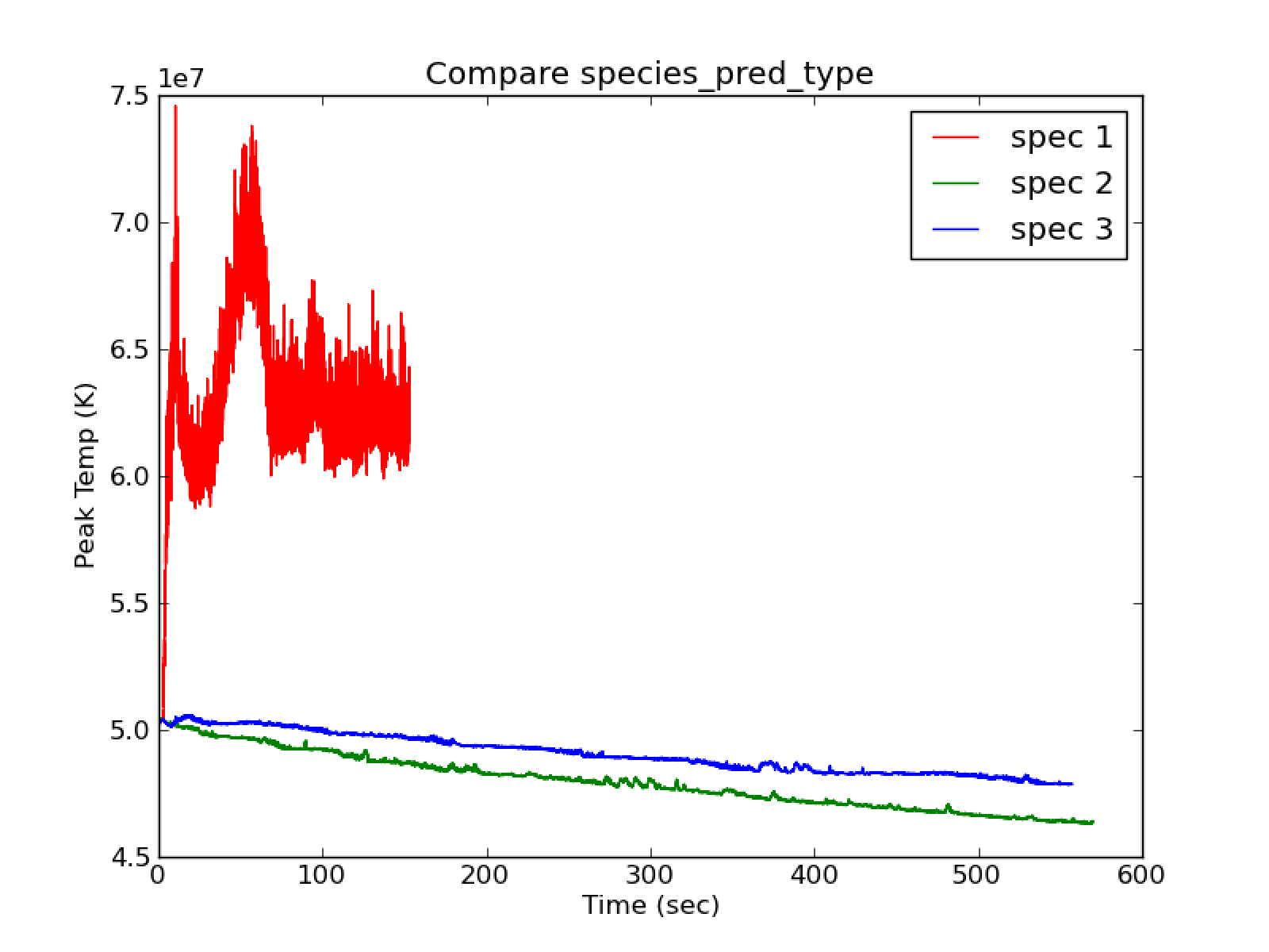
Fig. 18 Compare species_pred_type = 1,2,3 with use_tfromp = T, enthalpy_pred_type = 1, cflfac = 0.7

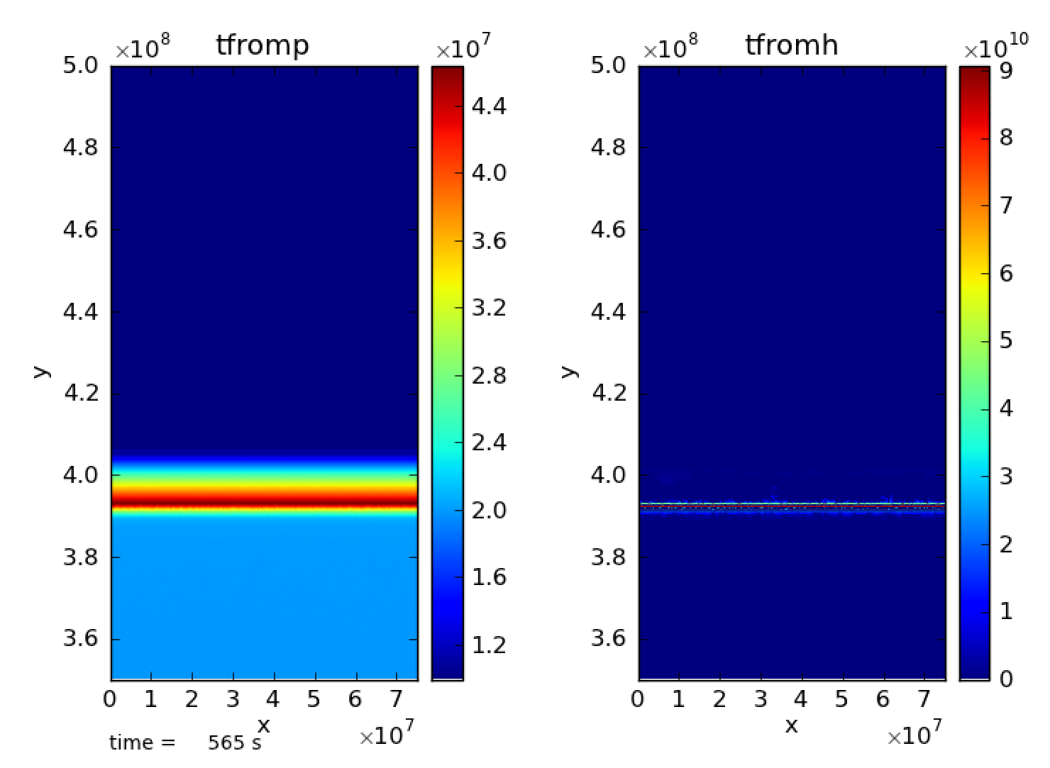
Fig. 19 There are strange filament type features at the bottom of the domain. species_pred_type = 2, enthalpy_pred_type = 1, cflfac = 0.7, use_tfromp = T

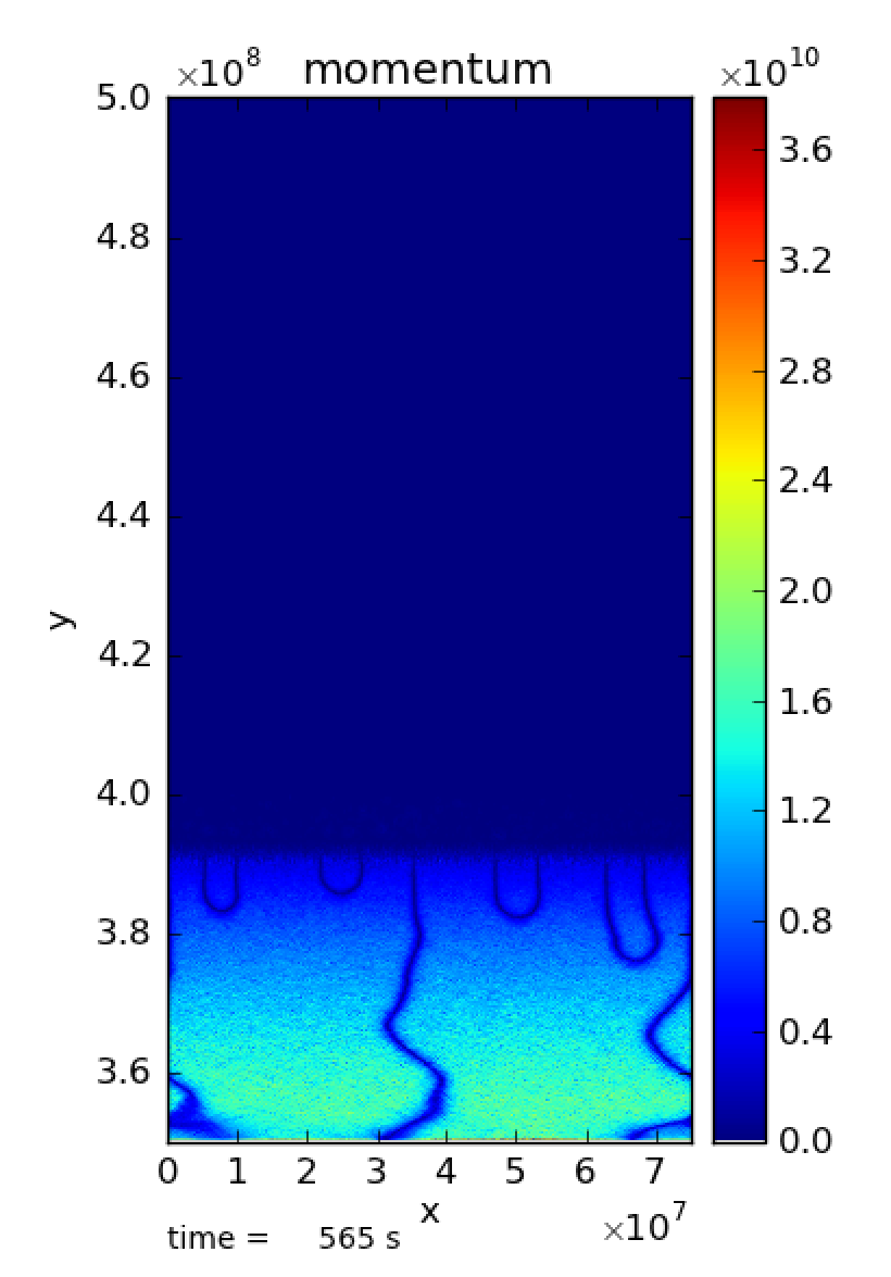
Fig. 20 There are strange filament type features at the bottom of the domain. species_pred_type = 2, enthalpy_pred_type = 1, cflfac = 0.7, use_tfromp = T

Using use_tfromp = F and dpdt_factor \(>\) 0 results in many runs crashing very quickly and gives unphyiscal temperature profiles as seen in Fig. 21.

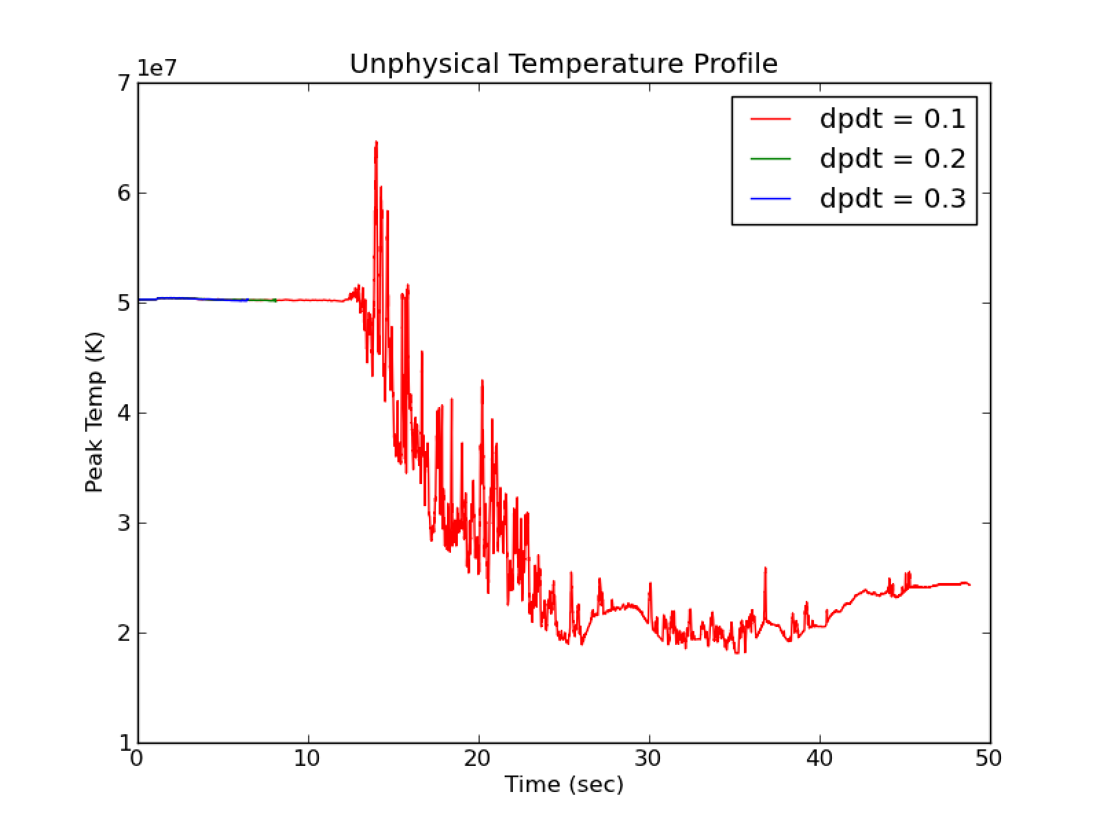
Fig. 21 Compare cflfac = 0.1 with cflfac = 0.7 for use_tfromp = F, dpdt_factor = 0.0, species_pred_type = 2, enthalpy_pred_type = 4

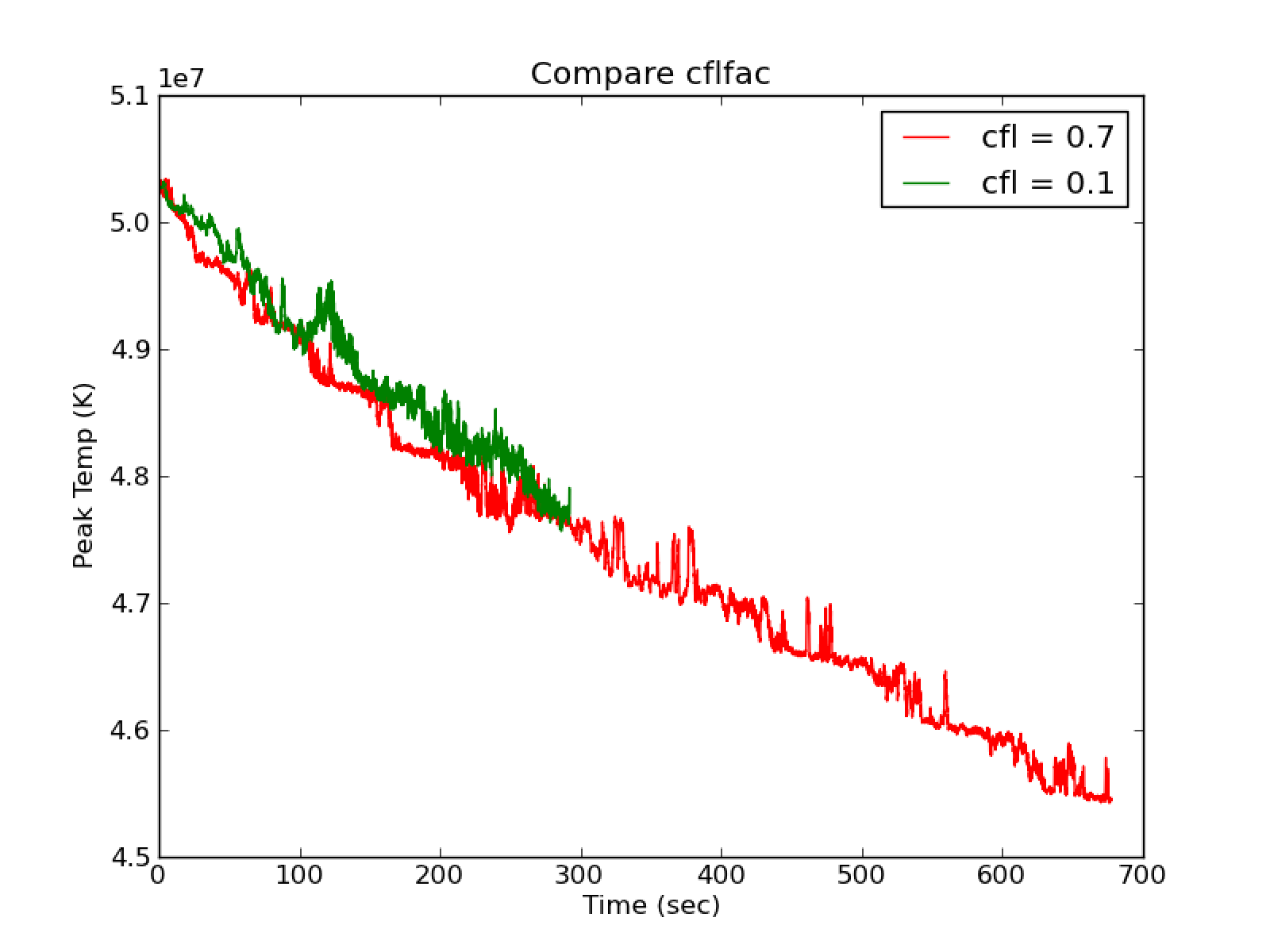
Fig. 22 Compare cflfac = 0.1 with cflfac = 0.7 for use_tfromp = F, dpdt_factor = 0.0, species_pred_type = 2, enthalpy_pred_type = 4

Change cflfac and enthalpy_pred_type

With species_pred_type = 1 and cflfac = 0.1, there is much less heating (peak T vs. t) than the cflfac = 0.7 (default). There is also a lower overall Mach number (see Fig. 23) with the cflfac = 0.1 and excellent agreement between tfromh and tfromp.

use_tfromp = F, dpdt_factor = 0.0, enthalpy_pred_type = 3,4 and species_pred_type = 2,3 shows cooling (as seen in use_tfromp = T) with a comparable rate of cooling (see Fig. 24) to the use_tfromp = T case. The largest difference between the two runs is that the use_tfromp = F case shows excellent agreement between tfromh and tfromp with cflfac = 0.7. The filaments in the momentum plot of Fig. 20 are still present.

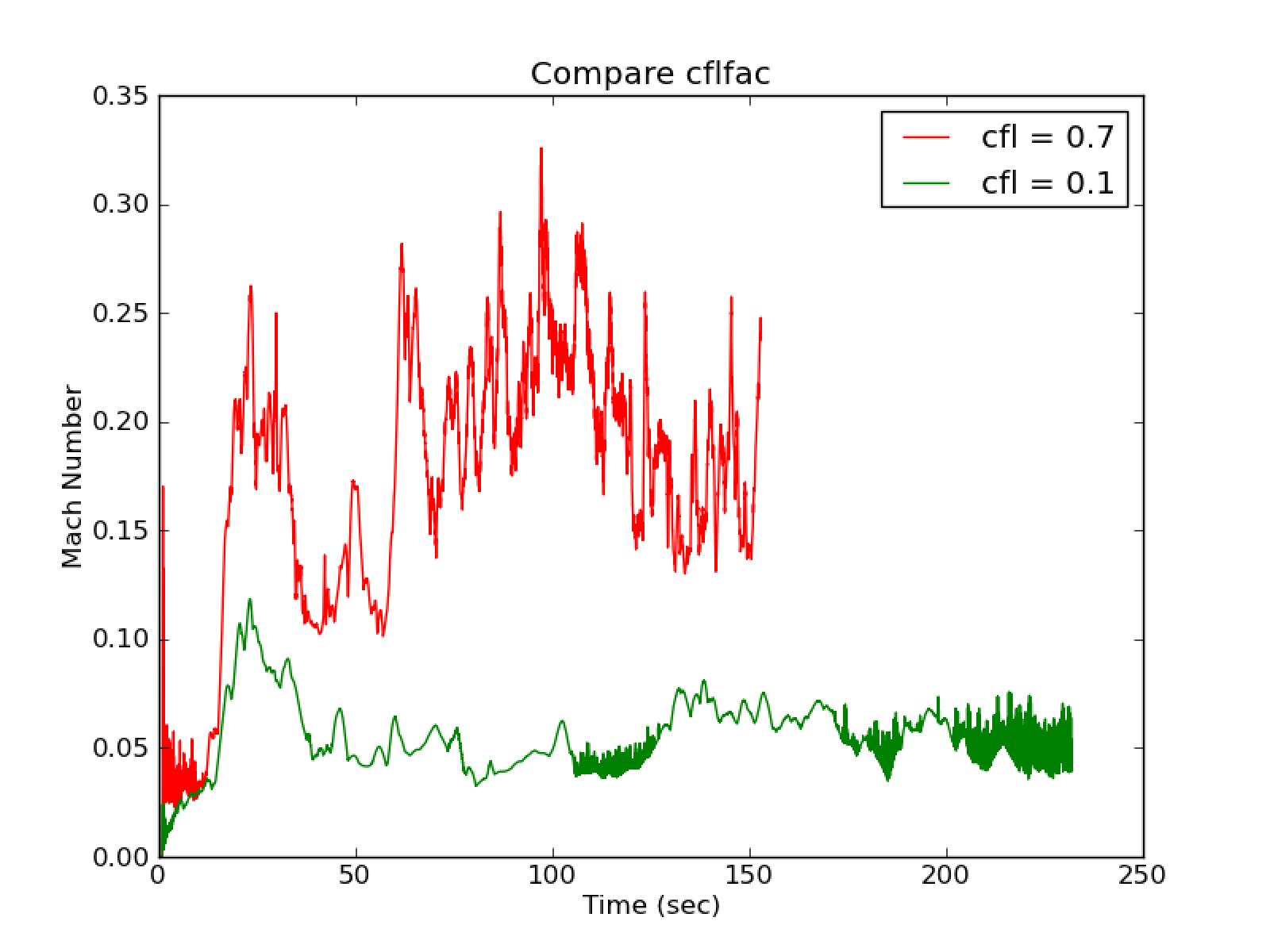
Fig. 23 Illustrate the comparable cooling rates between use_tfromp = T and use_tfromp = F with dpdt_factor = 0.0 using species_pred_type = 2, enthalpy_pred_type = 3,1

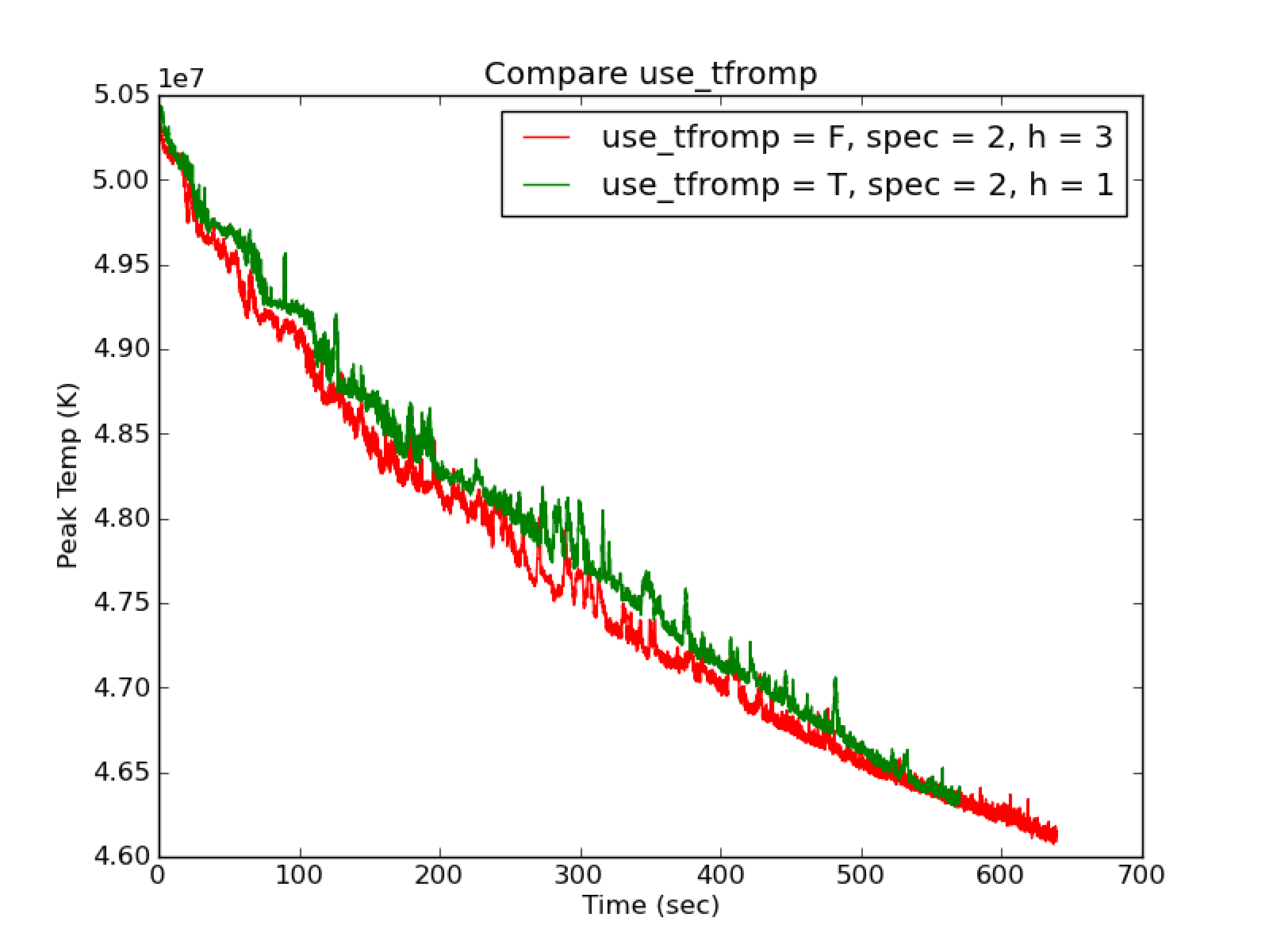
Fig. 24 Illustrate the comparable cooling rates between use_tfromp = T and use_tfromp = F with dpdt_factor = 0.0 using species_pred_type = 2, enthalpy_pred_type = 3,1

For a given enthalpy_pred_type and use_tfromp = F, species_pred_type = 2 has a lower Mach number (vs. t) compared to species_pred_type = 3.

Any species_pred_type with use_tfromp = F, dpdt_factor = 0.0 and enthalpy_pred_type = 1 shows significant heating, although the onset of the heating is delayed in species_pred_type = 2,3 (see Fig. 25). Only species_pred_type = 1 gives good agreement between tfromh and tfromp.

Comparing cflfac = 0.7 and cflfac = 0.1 with use_tfromp = F, dpdt_factor = 0.0, species_pred_type = 2 and enthalpy_pred_type = 4 shows good agreement overall (see Fig. 22.

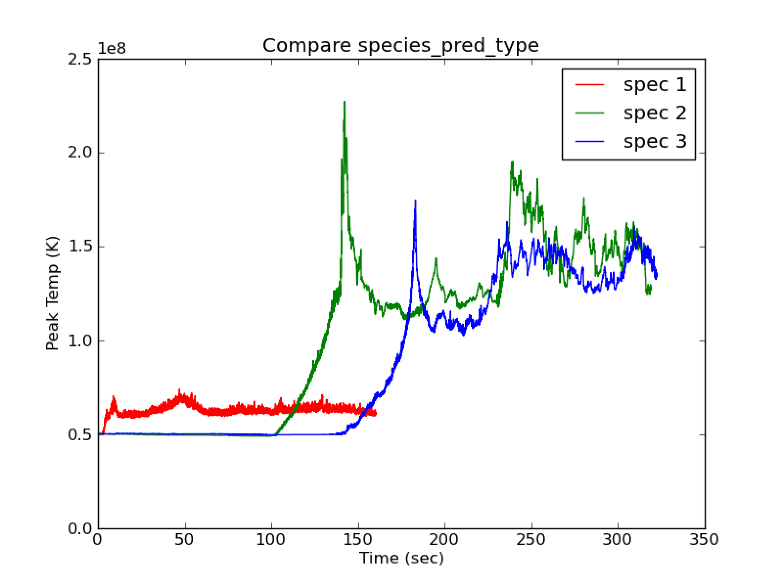
Fig. 25 Compare the castro.ppm_type CASTRO runs with the species_pred_type MAESTROeX runs.

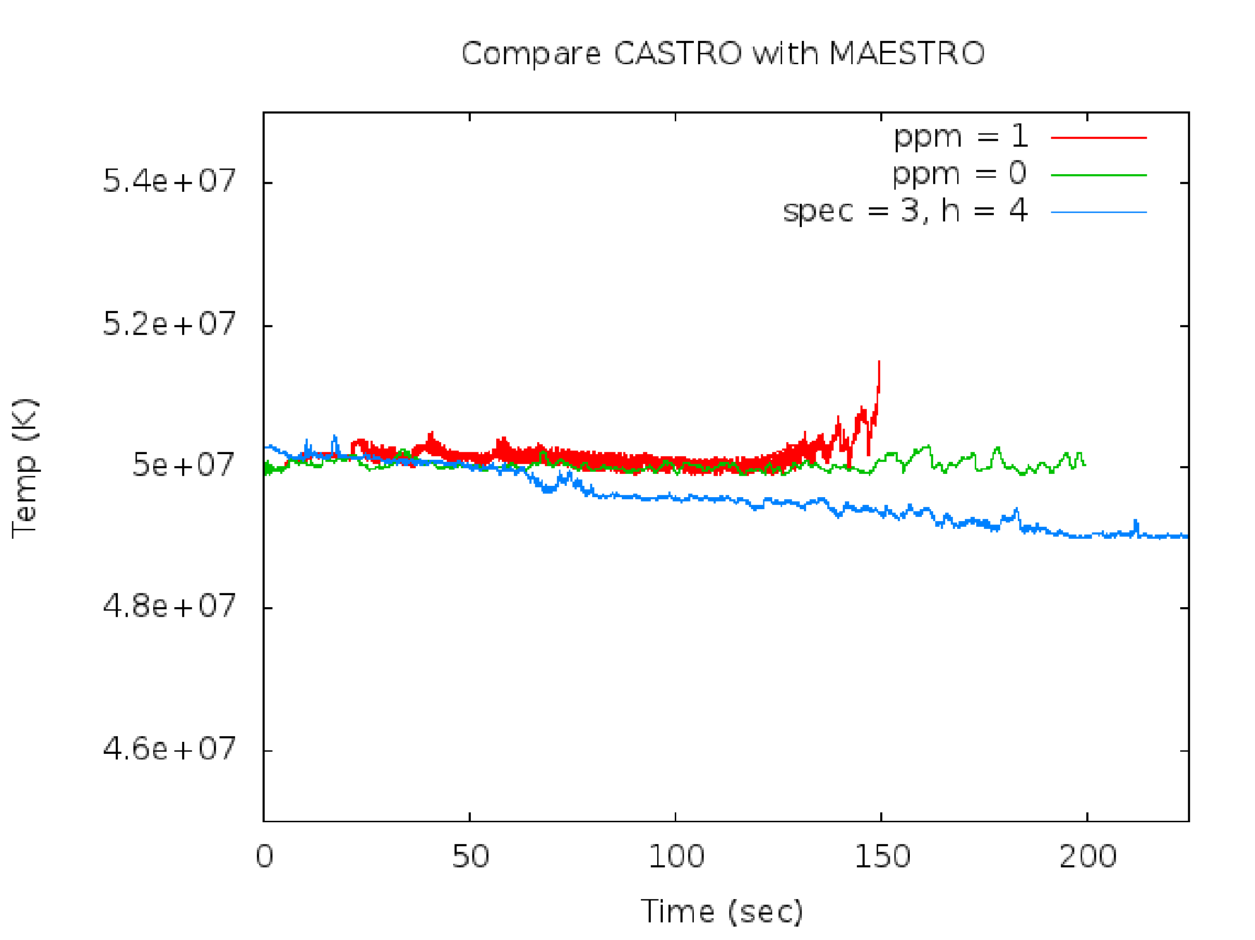
Fig. 26 Compare the castro.ppm_type CASTRO runs with the species_pred_type MAESTROeX runs.

Additional Runs

bds_type = 1

Using bds_type = 1, use_tfromp = F, dpdt_factor = 0.0, species_pred_type = 2, enthalpy_pred_type = 4 and cflfac = 0.7 seems to cool off faster, perhaps due to less mixing. There is also no momentum filaments in the bottom of the domain.

evolve_base_state = F

Using evolve_base_state = F, use_tfromp = F, dpdt_factor = 0.0, species_pred_type = 2 and enthalpy_pred_type = 4 seems to agree well with the normal evolve_base_state = T run.

toy_convect in CASTRO

toy_convect was also run using CASTRO with castro.ppm_type = 0,1. These runs show temperatures that cool off rather than increase (see Fig. 26) which suggests using species_pred_type = 2,3 instead of species_pred_type = 1.

Recommendations

All of these runs suggest that running under species_pred_type = 2 or 3, enthalpy_pred_type = 3 or 4 with either use_tfromp = F and dpdt_factor = 0.0 or use_tfromp = T gives the most consistent results.